Algebraic surfaces

Abstract.

This document includes notes for a 16-hour TCC course I taught in the autumn of 2024 on algebraic surfaces. None of this content is original to me. Almost all the facts here can be found in the excellent texts by Beauville and Reid. The goal is to state the Enriques–Kodaira classification in characteristic 0. Of course, any errors here should be marked down to me.

1. Some motivation

Standing assumption.

$k=\overline{k}$ is an algebraically closed field of characteristic $0$. You will lose absolutely nothing by assuming $k=ℂ$.

This course is ostensibly about birational geometry (though probably we’ll spend more time on other stuff). In particular, we are really want to understand the function field $k(X)$ where $X$ is an irreducible variety.

Definition 1.1.

If $X/k$, $Y/k$ are irreducible varieties, we say that $X$ and $Y$ are birational if $k(X)\cong k(Y)$.

Question 1.2.

Given $X,Y$ irreducible varieties over $k$, can we tell if $X$ and $Y$ are birational?

We want to associate invariants (i.e., numbers) to $X$ and $Y$ which allow us to tell them apart. The first one you probably already know.

Definition 1.3.

If $X/k$ is irreducible, the dimension of $X$ is the transcendence degree of $k(X)/k$.

It is clear that the dimension is a birational invariant. We break down by dimension.

1.1. Dimension 0

Over an algebraically closed field there is nothing to say about points, they’re points.

1.2. Dimension 1

We will need to say a lot about curves to study surfaces. Let $X/k$ be an irreducible variety of dimension $1$. There is a very useful fact about curves

Lemma 1.4.

There exists a unique smooth projective curve $\tilde{X}$ birational to $X$.

From the lemma, to study curves up to birational equivalence it suffices to study smooth projective curves up to isomorphism! This is very convinient. In particular we have a very nice isomorphism invariant (if $k=ℂ$).

Definition 1.5.

Define the geometric genus of $\tilde{X}$ to be the genus of the associated Riemann surface $\tilde{X}(ℂ)$.

Remark 1.6.

Actually, it really is enough to define the genus over $ℂ$. The field of definition of $\tilde{X}$ has finite transcendence degree over $\mathbb{Q}$ (even if $k$ is huge, $\tilde{X}$ is cut out by finitely many equations on finitely many affines) and therefore embeds in $ℂ$. This is an example of the Lefschetz Principle.

In any case, we’ll later see how to define the genus without reference to the Riemann surface $\tilde{X}(ℂ)$.

The genus is a really good invariant. One reason is that for each $g\ge 0$ there exists an irreducible variety of moduli ${ℳ}_g$ whose $ℂ$-points are in bijective correspondence with $ℂ$-isomorphism classes of curves of genus $g$.

1.3. Dimension 2

I am claiming that we can do an entire course on this case, so hopefully it’s quite a bit harder. Here’s a bunch of questions:

Question 1.7.

Let $X/k$ be an irreducible variety of dimension $2$:

1. Can we tell if $k(X)\cong k(t_1,t_2)$?

2. Does there exist a “good” choice of model for $X$?

3. Can we get a “curvature trichotomy”-esque invariant?

The answer is yes (Castelnovo’s rationality criterion), yes (in the non-ruled case we have the minimal model), and yes (the Kodaira dimension).

2. Housework

Let $X/k$ be an irreducible variety (in particular $X$ is also reduced). Let $U$ be any open affine subvariety of $X$ i.e., so that $U\cong \mathrm{Spec}A$ for some $k$-algebra $A$. Since $X$ is irreducible (and reduced) the ring $A$ is an integral domain. The function field $k(X)$ of $X$ is defined to be the fraction field of $A$.

Remark 2.1.

If you prefer to minimise scheme words, you could find $U$ so that $U$ is a Zariski open subset of $𝕍(f_1,\mathrm{\dots },f_m)\subset {𝔸}^n$ and then take

$$k(X)=\mathrm{Frac}k[t_1,\mathrm{\dots },t_n]/(f_1,\mathrm{\dots },f_m).$$

Figure 1. Prime divisors on a surface and a curve.

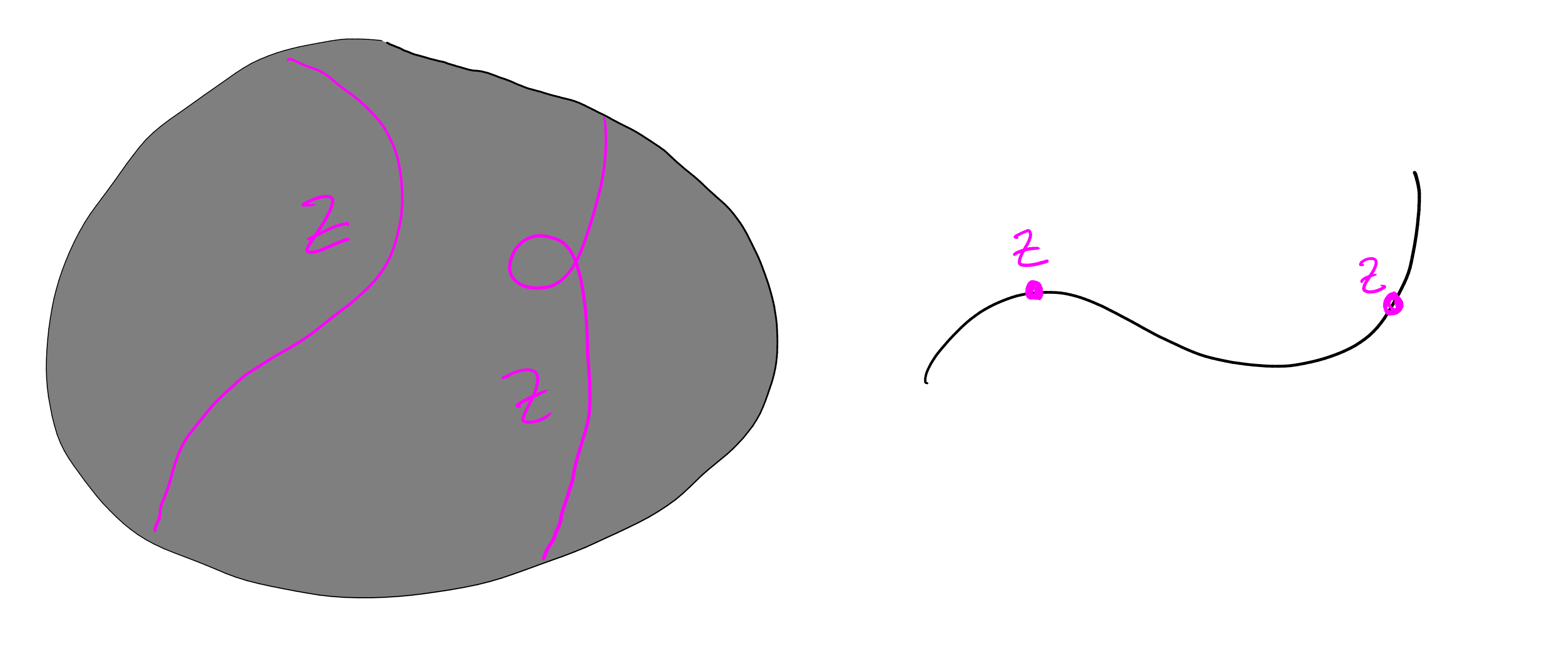
Definition 2.2.

Let $X$ be a smooth irreducible variety. A Weil divisor is a finite formal sum

$$D=\sum _Z{n}_Z\cdot Z$$

where the sum ranges over prime divisors (closed irreducible subvarieties $Z⊊X$ of codimension $1$). Write $\mathrm{Div}(X)$ for the free abelian group supported on the prime divisors.

We say $D$ is effective (written $D\ge 0$) if $n_Z\ge 0$ for all $Z$.

A note on sketches.

I am not a capable artist, and this is evidenced by the fact that I cannot accurately draw $4$-dimensional manifolds over $ℝ$. I compromise by drawing the real points of complex surfaces. Similarly, I am bad at drawing open sets in the Zariski topology – you will have to re-imagine my usual-complex-topology open sets.

If $Z\subset X$ is a prime divisor we can choose some open affine $U\subset X$ for which $U\cap Z\ne \mathrm{\varnothing }$, say $U\cong \mathrm{Spec}A$. Then $U\cap Z$ is isomorphic to a closed irreducible subvariety of $\mathrm{Spec}A$ and therefore we have $U\cap Z\cong \mathrm{Spec}A/𝔭$ for some prime ideal $𝔭\subset A$ (i.e., $U\cap Z$ is cut out by the polynomials in $𝔭$). Since $Z$ has codimension $1$ the ideal $𝔭$ has “height 1” and therefore the local ring

$${𝒪}_{X,Z}=A_{𝔭}\subset k(X)$$

is a DVR and comes equipped with a discrete valuation

$$v_Z:{𝒪}_{X,Z}\twoheadrightarrow {\mathbb{Z}}_{\ge 0}$$

which then extends to a valuation

$$v_Z:k(X)\to \mathbb{Z}$$

which “picks outthe order of vanishing of a rational function along $Z$”.

Example 2.3.

Take $X={\mathbb{P}}^1$ and $f=t_1=x_1/x_0$. For each $a\in k$ let $P=[1:a]$. We have ${𝒪}_{X,\mathrm{\infty }}=k{[t_1]}_{(t_1-a)}$ and $v_P$ picks out the power of $t_1-a$ in the numerator of $f$. Thus

At $\mathrm{\infty }$ we have to use the transition functions. Take $u_0=x_0/x_1$. Then we have $f=1/u_0$, so that $v_{\mathrm{\infty }}(f)=-1$.

Exercise 2.4.

More generally let $X={\mathbb{P}}^n$ and let $F\in k[x_0,\mathrm{\dots },x_n]$ be a homogeneous polynomial of degree $d$. Take $f=F/x_0^d\in k(X)$, let $Z=𝕍(F)$, and let $H=𝕍(x_0)$ be the hyperplane at infinity. Show that

Remark 2.5.

Often people write ${𝒪}_{X,\xi }$ where $\xi$ is the generic point of $Z$ and ${𝒪}_{X,\xi }$ is the stalk of the structure sheaf at $\xi$.

Exercise 2.6.

Check that the preceding definitions do not depend on the choice of open affine.

Definition 2.7.

For $f\in k{(X)}^{\times }$ define the divisor of zeroes and poles of $f$

$$\mathrm{div}(f)=\sum _Z{v}_Z(f)\cdot Z.$$

We say that a pair of Weil divisors $D,D^{\prime }\in \mathrm{Div}(X)$ are linearly equivalent (write $D\sim D^{\prime }$) if $D-D^{\prime }=\mathrm{div}(f)$ for some $f\in k{(X)}^{\times }$.

Definition 2.8.

If $X/k$ is a smooth, projective, irreducible variety we define the Picard group $\mathrm{Pic}(X)=\mathrm{Div}(X)/\sim$. For a Weil divisor $D$ we write $[D]$ for the class of $D$ in $\mathrm{Pic}(X)$.

Remark 2.9.

The experts will notice that I’ve imposed enough assumptions in the previous definition to ensure that Cartier divisors talk to linear equivalence classes of Weil divisors, if $X$ is subject to fewer hypotheses (in particular if you need to relax smoothness) you should be more careful.

Example 2.10.

Continuing from Exercise 2.4. We have

$$\mathrm{div}(f)=Z-dH.$$

Thus $Z\sim dH$ and therefore $\mathrm{Pic}(X)\cong \mathbb{Z}$ (take $[H]↤1$).

Exercise 2.11.

Show that $\mathrm{Pic}({\mathbb{P}}^1\times {\mathbb{P}}^1)\cong \mathbb{Z}\times \mathbb{Z}$ generated by $H\times \{\text{pt}\}$ and $\{\text{pt}\}\times H$.

2.1. Differentials and canonical divisors

The goal is to pluck out a “canonical divisor” of a projective variety $X/k$. Here there is an incomplete treatment but please see Shafarevich’s book [5, Chapter 3.5] for something much better.

Try 1:  Try the divisor $\mathrm{div}(f)$ for some $f\in k{(X)}^{\times }$. This is no good, because we’ve already used this to define linear equivalence.

Try 2:  Consider some projective embedding $X\hookrightarrow {\mathbb{P}}^n$, and take a hyperplane section. This is ok, but it depends on the extrinsic data of an embedding.

Try 3:  Differentials.

Definition 2.12.

A rational $1$-form is an expression

$$gdff,g\in k(X)$$

subject to the Leibniz rules

• $da=0$ for all $a\in k$,

• $𝑑(f+g)=df+dg$ for all $f,g\in k(X)$,

• $𝑑(fg)=fdg+gdf$ for all $f,g\in k(X)$.

We write ${\mathrm{\Omega }}_{k(X)/k}$ for the $k(X)$-module of rational $1$-forms.

Lemma 2.13.

If $f_1,\mathrm{\dots },f_n\in k(X)$ is a transcendence basis for $k(X)/k$, then ${\mathrm{\Omega }}_{k(X)/k}$ is generated as a $k(X)$-module by $d{f}_1,\mathrm{\dots },d{f}_n$.

Proof.

Exercise. ∎

Example 2.14.

1. $X={\mathbb{P}}^1$ so that $k(X)=k(t_1)$. Then ${\mathrm{\Omega }}_{k(X)/k}=\{gd{t}_1:g\in k(X)\}$.

2. $X=𝕍(x_0{x}_2^2+x_1^3+x_0^3)\subset {\mathbb{P}}^2$. Then ${\mathrm{\Omega }}_{k(X)/k}=\{gd{t}_1:g\in k(X)\}$.

3. $X={\mathbb{P}}^n$. Then ${\mathrm{\Omega }}_{k(X)/k}=\{g_{1}d{t}_1+\mathrm{\dots }+g_{n}d{t}_n:g\in k(X)\}$.

2.1.1. Canonical divisor on a curve

Start with curves (irreducible dimension $1$ varieties).

Definition 2.15 (Divisor of a $1$-form on a curve).

Let $X/k$ be a smooth projective curve and non-zero $s\in {\mathrm{\Omega }}_{k(X)/k}$. For each $P\in X(k)$ choose non-constant $f\in k(X)$ so that $v_P(f)=1$ (a “uniformiser”), then $s=gdf$ for some $g\in k(X)$. Define $v_P(s)=v_P(g)$ and

$$\mathrm{div}(s)=\sum _P{v}_P(s)\cdot P.$$

Example 2.16.

Let $X={\mathbb{P}}^1$ and $s=d{t}_1$. For all $a\in k$ we have $s=d{t}_1=d(t_1-a)$ so that $v_P(s)=v_P(1)=0$ for all $P=(1:a)$. At $\mathrm{\infty }=(0:1)$ we have $s=d{t}_1=d(1/t_0)=-t_0^{-2}d{t}_0$. In particular $v_{\mathrm{\infty }}(d{t}_0)=-2$ and $\mathrm{div}(s)=-2(\mathrm{\infty })$.

This seems pretty promising (it’s at least not linearly equivalent to $0$!).

Definition 2.17.

Let $X/k$ be a smooth projective curve. A canonical divisor $K_X$ for $X$ is any divisor of the form $\mathrm{div}(s)$ for some non-zero $s\in {\mathrm{\Omega }}_{k(X)/k}$.

One should very much hope that this divisor is actually well defined… good news.

Lemma 2.18.

Let $X/k$ be a smooth projective curve. The linear equivalence class of $K_X$ does not depend on the choice of rational $1$-form.

2.1.2. More general

An important input in Definition 2.17 is that by Lemma 2.13 there is a $1$-dimensional space of $1$-forms on a curve. We need to get that back when the dimension is $>1$. The idea is to take top wedge powers.

Recall that if $V/K$ is a vector space, for each $p\ge 1$ we have

$${\bigwedge }^{p}V=\left({⨂}^{p}V\right)/R$$

where $R=\mathrm{span}\{v_1\otimes \mathrm{\dots }\otimes v_p:v_i=v_j\text{ for some }i\ne j\}$. The following properties are very useful when you want to compute anything with $p$-forms.

Proposition 2.19.

We have:

1. $v_1\wedge \mathrm{\dots }\wedge v_p=0$ if and only if $v_1,\mathrm{\dots },v_p$ are linearly dependent,

2. for a transposition $\sigma \in S_p$ we have $v_1\wedge \mathrm{\dots }\wedge v_p=-v_{\sigma (1)}\wedge \mathrm{\dots }\wedge v_{\sigma (p)}$, and

3. if ${dim}_{K}V=n$ then ${dim}_K{\bigwedge }^{n}V=1$ and ${\bigwedge }^{n}V$ is spanned by $e_1\wedge \mathrm{\dots }\wedge e_n$ for any basis $\{e_1,\mathrm{\dots },e_n\}$ of $V$.

Corollary 2.20.

If $dimX=n$ then the space ${\mathrm{\Omega }}_{k(X)/k}^n:={\bigwedge }^n{\mathrm{\Omega }}_{k(X)/k}$ of rational $n$-forms is a $k(X)$-vector space of dimension $1$.

With Corollary 2.20 in our pocket, we are in with a shout of being able to define something reasonable as a canonical divisor.

To get to another $n$-form we only need to multiply by a rational function – so any good definition of divisor of an $n$-form will make two divisors-of-$n$-forms differ by the divisor of a rational function!

Let $X/k$ be a smooth, irreducible, projective variety of dimension $n$. Recall that at a point $P\in X$ we say $z_1,\mathrm{\dots },z_n\in k{(X)}^{\times }$ are local coordinates at $P$ if $z_1,\mathrm{\dots },z_n$ span the cotangent space ${𝔪}_P/{𝔪}_P^2$ (where here ${𝔪}_P$ is the maximal ideal of the local ring ${𝒪}_{X,P}$).

Example 2.21.

If $X={𝔸}^n$ and $P\in X$ is the origin, then ${𝒪}_{X,P}=k{[t_1,\mathrm{\dots },t_n]}_{{𝔪}_P}$ where ${𝔪}_P=(t_1,\mathrm{\dots },t_n)$. In particular the coordinates $t_1,\mathrm{\dots },t_n$ are local coordinates.

Now take $s\in {\mathrm{\Omega }}_{k(X)/k}^n$, a non-zero rational $n$-form. Let $Z\subset X$ be a prime divisor and choose $z_1,\mathrm{\dots },z_n\in k{(X)}^{\times }$ to be local coordinates for at (any point in) an open $U\subset X$ for which $Z\cap U\ne \mathrm{\varnothing }$. Further suppose that $z_1,\mathrm{\dots },z_n$ are regular on $U$ (we can always achieve this by shrinking $U$ if necessary). Then by Corollary 2.20 $s=gd{z}_1\wedge \mathrm{\dots }\wedge d{z}_n$ for some rational function $g\in k{(X)}^{\times }$. We define

$$v_Z(s)=v_Z(g).$$

Remark 2.22.

In practice, to compute the valuation of $s\in {\mathrm{\Omega }}_{k(X)/k}^n$ along every prime divisor one only needs to cover $X$ with finitely many open sets because $X$ is quasi-compact in the Zariski topology.

Exercise 2.23.

The definition of $v_Z(s)$ above does not depend on the choice of open set $U$, nor the choice of local coordinates $z_1,\mathrm{\dots },z_n$.
Hint: cover $X$ in open affines (one for each point, and small enough so that your favourite local coordinates on each are regular) and compare pairs of volume forms $d{z}_1\wedge \mathrm{\dots }\wedge d{z}_n$ and $d{\zeta }_1\wedge \mathrm{\dots }\wedge d{\zeta }_n$ by showing that the Jacobian determinant $J=\left|\frac{\partial {\zeta }_i}{\partial z_j}\right|$ is non-vanishing and regular on overlaps.

Definition 2.24.

Let $X/k$ be a smooth, irreducible, projective variety and let $s\in {\mathrm{\Omega }}_{k(X)/k}^n$ be a non-zero rational $n$-form. We define the divisor of $s$ to be

$$\mathrm{div}(s)=\sum _Z{v}_Z(s)Z$$

where the sum ranges over the prime divisors of $X$.

Of course, the first thing we should show is the important lemma.

Lemma 2.25.

Let $X/k$ be a smooth, irreducible, projective variety. Then linear equivalence class of the divisor $K_X=\mathrm{div}(s)$ of a rational $n$-form $s\in {\mathrm{\Omega }}_{k(X)/k}^n$ does not depend on the choice of $s$. We call $K_X$ a canonical divisor on $X$.

Example 2.26.

Let $X={\mathbb{P}}^2$, write $t_1=x_1/x_0$ and $t_2=x_2/x_0$. Take $s=d{t}_1\wedge d{t}_2\in {\mathrm{\Omega }}_{k(X)/k}^2$. Now clearly $s$ has no zeroes or poles on the patch with $x_0\ne 0$. Then swapping patches by setting $u_0=x_0/x_2$ and $u_1=x_1/x_2$ so that $t_1=u_1/u_0$ and $t_2=1/u_0$ we have

$d{t}_1\wedge d{t}_2$ $=d(u_1/u_0)\wedge d(1/u_0)$

$={\displaystyle \frac{u_{0}d{u}_1-u_{1}d{u}_0}{u_0^2}}\wedge {\displaystyle \frac{-d{u}_0}{u_0^2}}$

$={\displaystyle \frac{-d{u}_1\wedge d{u}_0}{u_0^3}}-{\displaystyle \frac{u_{1}d{u}_0\wedge d{u}_0}{u_0^4}}$

$={\displaystyle \frac{-d{u}_1\wedge d{u}_0}{u_0^3}}$

$={\displaystyle \frac{1}{u_0^3}}d{u}_0\wedge d{u}_1.$

Therefore writing $H=𝕍(x_0)$ we have $v_H(s)=-3$ and therefore $\mathrm{div}(s)=-3H$. In particular $K_{{\mathbb{P}}^2}\sim -3H$.

Actually this is more general.

Lemma 2.27.

We have $K_{{\mathbb{P}}^n}\sim -(n+1)H$ where $H=𝕍(x_0)$ (or any hyperplane, for that matter).

Proof.

Exercise, follow your nose as above. ∎

Exercise 2.28.

Show that if $X={\mathbb{P}}^1\times {\mathbb{P}}^1$ then $K_X\sim -2H-2H^{\prime }$ where $H=\{\text{pt}\}\times {\mathbb{P}}^1$ and $H^{\prime }={\mathbb{P}}^1\times \{\text{pt}\}$.

Again, there is a more general form of Exercise 2.28.

Lemma 2.29.

Let $X=Y_1\times Y_2$ and let ${\pi }_i:X\to Y_i$ be the projection onto the $i^{\text{th}}$ factor, then $K_X\sim {\pi }_1^{\ast }{K}_{Y_1}+{\pi }_2^{\ast }{K}_{Y_2}$.

Proof.

Exercise. ∎

Remark 2.30.

Later we will prove the adjunction formula (Theorem 5.9) which will allow us to get a canonical divisor on a complete intersection by making adjustments, then intersecting with subvarieties.

3. Curves

By a smooth curve I mean a smooth irreducible (reduced) projective variety $X/k$ of dimension $1$. Remember, the question we’re asking is:

Question 3.1.

How do we distinguish curves?

Try 1:  Consider the space $H^0(X,{𝒪}_X)$ of everywhere regular rational functions $f\in k(X)$. But there is the well known lemma.

Lemma 3.2.

Let $X/k$ be an irreducible proper (e.g., projective) variety. Then $H^0(X,{𝒪}_X)\cong k$.

So unfortunately this can’t give us a good number.

Remark 3.3.

When $k=ℂ$ and $X={\mathbb{P}}^1$ one should compare this to Liouville’s theorem (every bounded holomorphic function $ℂ\to ℂ$ is constant – bounded means there is no pole at infinity). More generally when $k=ℂ$ one can use compactness and the maximum modulus principle.

Try 2:  Let $D$ be a Weil divisor on $X$. Consider the space

$$H^0(X,{𝒪}_X(D))=\{f\in k{(X)}^{\times }:\mathrm{div}(f)+D\ge 0\}\cup \{0\}$$

of rational functions with “poles allowed by $D$ and zeroes forced by $D$”. From this we can get a number, namely $h^0(X,{𝒪}_X(D))={dim}_k{H}^0(X,{𝒪}_X(D))$ (in general little $h$ is the dimension of big $H$).

Example 3.4.

Let $X={\mathbb{P}}^1$ and take $D=n(\mathrm{\infty })$. Then

$$H^0(X,{𝒪}_X(D))=\{f\in k[t_1]:\mathrm{deg}(f)\le n\}.$$

In particular $h^0(X,{𝒪}_X(D))=n+1$ (the number of monomials).

Try 3:  The problem with try 2 is of course that we have to name a divisor. But we have a way to do that!

Definition 3.5.

Define the geometric genus of $X$ to be $p_g(X)=h^0(X,{𝒪}_X(K_X))$.

Example 3.6.

Take $X={\mathbb{P}}^1$. Then we know $K_X\sim -2(\mathrm{\infty })$. Then $h^0(X,{𝒪}_X(K_X))=0$ because we’re asking for those everywhere regular functions (i.e., constants) which have (at least) a double zero at infinity. That’s enough to make anyone zero.

Example 3.7.

Take $X$ to be a smooth cubic curve in ${\mathbb{P}}^2$. By the adjunction formula Theorem 5.9 we will see that $K_X\sim {𝒪}_X$. Thus by Lemma 3.2 we have $p_g(X)=1$.

3.1. The Riemann–Roch theorem

We now state the Riemann–Roch theorem, which is a powerful tool for computing the dimensions $h^0({𝒪}_X(D)):=h^0(X,{𝒪}_X(D))$ for divisors $D$ on a smooth projective curve $X$.

Theorem 3.8 (Riemann–Roch).

Let $D$ be a divisor on a smooth irreducible projective curve $X/k$. Then

$$\underset{\text{want this}}{\underbrace{h^0({𝒪}_X(D))}}-\underset{\text{error term}}{\underbrace{h^0({𝒪}_X(K_X-D))}}=\underset{\text{simple constant}}{\underbrace{\mathrm{deg}D-p_g(X)+1}}.$$

Example 3.9.

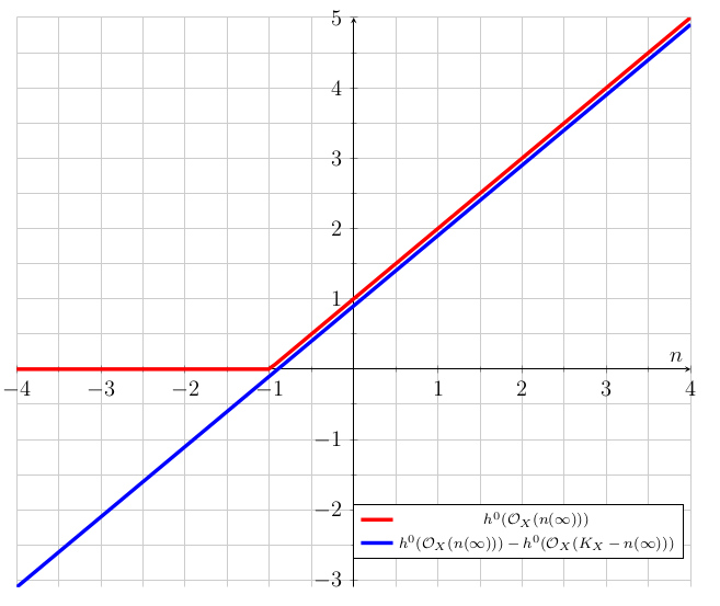
Continuing from Example 3.6 we know that $h^0({𝒪}_X(n(\mathrm{\infty })))=n+1=\mathrm{deg}(n(\mathrm{\infty }))+1$ whenever $n\ge 0$. But Riemann–Roch tells us that this should continue to happen when so long as we correct by the term $h^0({𝒪}_X(K_X-n(\mathrm{\infty })))$. But we have $K_X=-2(\mathrm{\infty })$ so this dimension is $h^0({𝒪}_X(E))$ where $E=(-n-2)(\mathrm{\infty })))$. Whenever $n\le -2$ we get $h^0({𝒪}_X(E))=(-n-2)+1=-n-1$ (as we want). When $n=-1$ we get that both $h^0({𝒪}_X(n(\mathrm{\infty })))$ and $h^0({𝒪}_X(E))$ are zero (as required, again). This example is illustrated in Figure 2.

Remark 3.10.

The point is that the correction term makes the dimensions “behave like linear functions in the degree”. Later we will see that this is really some manifestation of the Euler characteristic being the “right” thing to use in exact sequences when we want to find dimensions.

Figure 2. Riemann–Roch for ${\mathbb{P}}^1$ and $D=n(\mathrm{\infty })$. This kind of picture is made rigorous by the Hilbert polynomial.

Often Riemann–Roch is best used in the form of the following corollary.

Corollary 3.11.

We have:

1. $h^0({𝒪}_X(D))\le \mathrm{deg}D-p_g(X)+1$,

2. $\mathrm{deg}{K}_X=2p_g(X)-2$,

3. if $\mathrm{deg}D\ge 2p_g(X)-1$ then $h^0({𝒪}_X(K_X-D))=0$.

Proof.

(1) is clear. For (2) take $D=K_X$ then Riemann–Roch implies that $p_g(X)-1=\mathrm{deg}{K}_X-p_g(X)+1$ and the claim follows. For (3) combine (1) and (2) to obtain the bound $h^0({𝒪}_X(K_X-D))\le \mathrm{deg}(K_X-D)-p_g(X)+1\le \mathrm{deg}(K_X-D)+1\le 0$. ∎

I’ll conclude with a standard example of how to use Riemann–Roch.

Lemma 3.12.

Every genus $1$ curve $X/k$ (over an algebraically closed field) is isomorphic to a smooth cubic curve in ${\mathbb{P}}^2$.

Proof.

You can find something like this in [7, III]. Take a point $P\in X(k)$ (this is the only place we use the algebraic closure, actually). Now by Corollary 3.11 we have $\mathrm{deg}{K}_X=0$ and therefore we can compute

$$h^0({𝒪}_X(3P))=3\text{and}{h}^0({𝒪}_X(9P))=9.$$

But if we choose a basis $1,x,y\in H^0({𝒪}_X(3P))$ then each of the $10$ homogeneous degree $3$ monomials in $1,x,y$ lives in $H^0(𝒪(9P))$ (count the poles). In particular, there is a relation of degree $3$ between $1,x,y$.

Thus the rational map $\varphi :X⇢{\mathbb{P}}^2$ given by $[1:x:y]$ lands on a cubic curve $X^{\prime }$.

Exercise 3.13.

Check that $\varphi$ is in fact an isomorphism.

∎

Exercise 3.14.

Use a similar trick to show that every genus $1$ curve is isomorphic to an intersection of two quadrics in ${\mathbb{P}}^3$. Hint: consider $H^0({𝒪}_X(4P))$ and $H^0({𝒪}_X(8P))$.

4. Sheaves and stuff

This is not a course about sheaves, it’s more about using them. As such, I’m going to give a bunch of examples and if this section makes no sense at all, that’s ok. Anything I state you’re welcome to take as an axiom until you want to read Hartshorne. I quite like the short treatment in Reid’s notes [4, Chapter B], and I follow it relatively closely.

Example 4.1.

Let $X/k$ be an irreducible variety and take $U\subset X$ an open subset.

1. The structure sheaf ${𝒪}_X$ so that

   $$\mathrm{\Gamma }(U,{𝒪}_X)=\{f\in k{(X)}^{\times }:f\text{ is regular on }U\}\cup \{0\}.$$

2. If $X$ is smooth the sheaf ${𝒪}_X(D)$ for a Weil divisor $D$ so that

   $$\mathrm{\Gamma }(U,{𝒪}_X(D))=\{f\in k{(X)}^{\times }:\}.$$

3. If $X$ is smooth the sheaf of regular $1$-forms ${\mathrm{\Omega }}_{X/k}$ so that

   $$\mathrm{\Gamma }(U,{\mathrm{\Omega }}_{X/k})=\{s\in {\mathrm{\Omega }}_{X/k}:s\ne 0\text{ is regular on }U\}\cup \{0\},$$

   where regular means that there exist regular $f,g\in k(X)$ so that $s=gdf$.

4. If $X$ is smooth the sheaf of regular $p$-forms ${\mathrm{\Omega }}_{X/k}^p={\bigwedge }^p{\mathrm{\Omega }}_{X/k}$ so that

   $$\mathrm{\Gamma }(U,{\mathrm{\Omega }}_{X/k}^p)=\{s\in {\bigwedge }^p{\mathrm{\Omega }}_{X/k}:s\ne 0\text{ is regular on }U\}\cup \{0\},$$

   where regular means that there exist regular $g,f_1,\mathrm{\dots },f_p,\in k(X)$ so that $s=gd{f}_1\wedge \mathrm{\dots }\wedge d{f}_p$.

5. If $X$ is smooth, the canonical sheaf ${\omega }_X={\mathrm{\Omega }}_{X/k}^{dimX}$.

Obviously the $\mathrm{\Gamma }(U,{𝒪}_X)$ are rings, all the others are merely abelian groups. But actually, (2)–(4) are naturally $\mathrm{\Gamma }(U,{𝒪}_X)$-modules.

Definition 4.2 (Sketch definition).

A sheaf $ℱ$ of “foos” on a variety $X/k$ is some assignment which takes in open sets and spits out “foos” i.e., $U\mapsto \mathrm{\Gamma }(U,ℱ)$ (here “foos” are say sets, rings, abelian groups). To be a sheaf, there is additional data to make sure our sheaf encapsulate “function-ness”.

1. Given open sets $V\subset U\subset X$ there exist a restriction map ${\rho }_{UV}:\mathrm{\Gamma }(U,ℱ)\to \mathrm{\Gamma }(V,ℱ)$ which staisfies the condition that if $W\subset V\subset U$ then we have ${\rho }_{UW}={\rho }_{VW}\circ {\rho }_{UV}$.
   Slogan:  If you’re restricting the domain of a function it doesn’t matter if you first restrict a little less.

2. If you have something that looks like a function on an open cover of $U$, then it glues to a function on $U$ and you know it uniquely.

Exercise 4.3.

1. Look up the actual definition and check that my bad sketch is correct.

2. Come up with the definition of a sheaf of ${𝒪}_X$-modules (you want the restrictions to behave with the structure).

3. Come up with the definition of locally adjective.

Example 4.4 (Pushforward).

Let $i:Y\hookrightarrow X$ be a subvariety. We can “push-forward” a sheaf $ℱ$ on $Y$ to a sheaf $i_{\ast }ℱ$ on $X$ by defining

$\mathrm{\Gamma }(U,i_{\ast }ℱ)$ $=\mathrm{\Gamma }(U\cap Y,ℱ)$

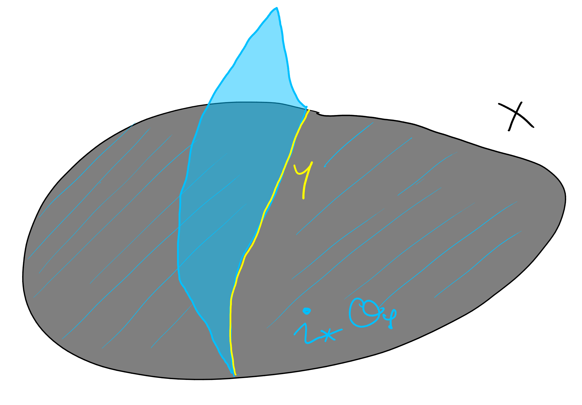
I like to think of this as a kind of “$\delta$-function” supported along $Y$.

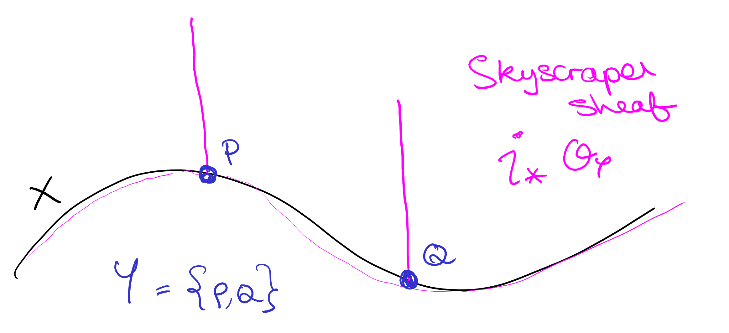
A typical example of this is the skyscraper sheaf. Take a finite set of (closed) points $Y=\{P_1,\mathrm{\dots },P_r\}\subset X(k)$ and consider $i_{\ast }{𝒪}_Y$. Since ${dim}_k\mathrm{\Gamma }(V,{𝒪}_Y)$ just counts the number of points in $V\subset Y$ one can think of $i_{\ast }{𝒪}_Y$ as some kind of indicator function for containing elements of $Y$. The name “skyscraper” comes from the vision on stalks – we get a $k$ at the stalks ${(i_{\ast }{𝒪}_Y)}_{P_i}$ and trivial everywhere else.

Figure 3. A sketch of what (I think) the stalks of the pushforward of the structure sheaf looks like. On the left is the skyscraper sheaf. Note that everything is supported along the “spine”.

Exercise 4.5.

Figure out what the skyscraper sheaf looks like when some of the points are non-reduced.

Exercise 4.6.

Define pushforward for any morphism $Y\to X$ (not just immersions).

We get to stalks. One should imagine this as the “algebraic-geometry-version-of-Taylor-series-expansions-of-holomorphic-functions”. That is, some kind of “very local” view of a function.

Definition 4.7.

Let $ℱ$ be a sheaf on a variety $X$. For a point $x\in X$ (here this could be a scheme-theoretic point i.e., non-closed) then the stalk of $ℱ$ at $x$ is defined as

$${ℱ}_x=\underset{⟶}{lim}\mathrm{\Gamma }(U,ℱ).$$

If this is intimidating, not to worry, you can take the following lemma as a definition.

Lemma 4.8.

Let $X$ be a variety and let $ℱ$ be a sheaf of ${𝒪}_X$-modules. Then for any affine open $\mathrm{Spec}A\cong U\ni x$. Identify $x$ with a prime ideal $𝔭\in \mathrm{Spec}A$, then

$${ℱ}_x=\mathrm{\Gamma }{(U,ℱ)}_{𝔭}$$

the localisation of $\mathrm{\Gamma }(U,ℱ)$ at $𝔭$.

Exercise 4.9.

Define $\otimes$ and quotients for sheaves. If you haven’t seen this before you’ll probably get it wrong, not to worry – this is a feature not a bug. The point is that we want these things to “look correct” on stalks, but then we may have to add in some “extra” sections to get the gluing to work.

Anyway, even if you don’t do the exercise the following should hopefully provide some orientation.

Proposition 4.10.

Let $X/k$ be an irreducible, smooth, projective variety and let $D,D^{\prime }$ be Weil divisors on $X$:

1. ${𝒪}_X(D)\cong {𝒪}_X(D^{\prime })$ if and only if $D\sim D^{\prime }$,

2. ${𝒪}_X(D){\otimes }_{{𝒪}_X}{𝒪}_X(D^{\prime })\cong {𝒪}_X(D+D^{\prime })$,

3. if $K_X$ is a canonical divisor on $X$ then ${\omega }_X\cong {𝒪}_X(K_X)$.

4.1. Exactness

The point here is that exactness is “hyper-local” in the sense that we want to be able to check it on stalks. Why not define it that way then!

Definition 4.11.

A sequence

$${ℱ}^{\prime }\to ℱ\to {ℱ}^{\prime \prime }$$

of sheaves of abelian groups on $X$ is exact if for every $x\in X$ the induced sequence

$${ℱ}_x^{\prime }\to {ℱ}_x\to {ℱ}_x^{\prime \prime }$$

of abelian groups is exact.

Example 4.12.

If we include a point $i:P\hookrightarrow X$ in a curve $X$ we have an exact sequence

$$0\to {𝒪}_X(-P)\to {𝒪}_X\to i_{\ast }{𝒪}_P\to 0.$$

It suffices to check this stalk-locally. If $x\ne P$ (closed) this is clear, since ${𝒪}_X{(-P)}_x={𝒪}_{X,x}$ and $i_{\ast }{({𝒪}_P)}_x=0$. If $x=P$ then $𝒪{(-P)}_P$ is the unique maximal ideal in ${𝒪}_{X,P}$ and ${(i_{\ast }{𝒪}_P)}_P=k$.

You will not lose much in this course if you take the following lemma only with closed subvarieties $Y\subset X$ (i.e., no reduced structure).

Lemma 4.13.

If $\iota :Y\hookrightarrow X$ is a closed subscheme of a variety $X/k$ then we have a short exact sequence

$$0\to {ℐ}_{Y|X}\to {𝒪}_X\to i_{\ast }{𝒪}_Y\to 0.$$

In particular, $X$ is smooth, projective, and irreducible then if $D$ is an effective divisor we have a short exact sequence

$$0\to {𝒪}_X(-D)\to {𝒪}_X\to i_{\ast }{𝒪}_D\to 0$$

where here we are abusively identifying $D$ and the corresponding pure codimension $1$ subscheme in $X$ (which is non-reduced if and only if $n_Z>1$ for some $Z$).

Proof.

Exercise, just check it on stalks. ∎

4.2. The failure of surjectivity

It turns out that when we take global sections, right exactness is not preserved. Let’s see a couple of examples.

Example 4.14.

Let $X={\mathbb{P}}^1$ and consider $Y=\{P,Q\}$ and let $D=P+Q$. Then $i_{\ast }{𝒪}_Y$ is the skyscraper sheaf supported on $P$ and $Q$. We have a short exact sequence

$$0\to {𝒪}_X(-D)\to {𝒪}_X\to i_{\ast }{𝒪}_Y\to 0.$$

But if we take global sections we have

This clearly cannot be surjective! The failure on the right is coming from the “error term” appearing in Riemann–Roch (the term $h^0({𝒪}_X(K_X-D))$).

Exercise 4.15.

Generalise Example 4.14 to more general curves $X$. Give a necessary and sufficient condition on $\mathrm{deg}D$ for the failure to occur.

Example 4.16.

I’ve borrowed this out of Reid’s notes. Take $X={\mathbb{P}}^n$ with $n\ge 2$ and take distinct points $P,Q,R\in X(k)$. Suppose for simplicity that $P,Q,R\notin H=𝕍(x_0)$ (for this example, we’ll be happy to move our hyperplane in its linear equivalence class anyway). Take $Y\subset X$ to be the three point variety $Y=\{P,Q,R\}$. We have the ideal sheaf exact sequence

$$0\to {ℐ}_{Y|X}\to {𝒪}_X\to i_{\ast }{𝒪}_Y\to 0.$$

The setup of this example is to tensor this exact sequence with ${𝒪}_X(H)$ – this tensoring preserves exactness by the global version of “free modules are flat”. So we have:

($\ast$) $$0\to {ℐ}_{Y|X}(H)\to {𝒪}_X(H)\to (i_{\ast }{𝒪}_Y)(H)\to 0.$$

I want to try describe the terms and the maps.

• A section $f\in \mathrm{\Gamma }(X,{𝒪}_X(H))$ is a “linear form” – a rational function of the sort $f=g/x_0$ where $g\in k[x_0,\mathrm{\dots },x_n]$ is linear.

• This is ${ℐ}_{Y|X}(H)={ℐ}_{Y|X}{\otimes }_{{𝒪}_X}{𝒪}_X(H)$. Then $\mathrm{\Gamma }(X,{ℐ}_{Y|X}(H))$ is exactly the set of linear forms which vanish on $Y$. The map ${ℐ}_{Y|X}(H)\to {𝒪}_X(H)$ is just inclusion.

• This is isomorphic to $i_{\ast }{𝒪}_Y({H|}_Y)=i_{\ast }{𝒪}_Y$ because $H$ does not meet $Y$.

• We have $\mathrm{\Gamma }(Y,{𝒪}_Y)\cong k^3$. The map says to take some function $f\in \mathrm{\Gamma }(X,{𝒪}_X(H))$ and evaluate it on $P$, $Q$, and $R$.

One can also see exactness of $(\ast )$ visually (without 4.13). Just go to a small enough affine open.

But now we want to take global section in $(\ast )$. Then we get

$$0\to \{\text{linear forms vanishing on }P,Q,R\}\to \mathrm{span}\{x_0,\mathrm{\dots },x_n\}\to k^3.$$

Now this is right exact so long as there is not an unexpected linear dependency – i.e., if they lie on a line! In the language of cohomology $H^1(X,{ℐ}_{Y|X}(H))\ne 0$ if our three points are colinear. All of this is controlled by an exact sequence

4.3. Cohomology of coherent sheaves

The idea for “fixing” these right exactness issues is to consider exact sequences of cohomology groups instead. We’ll probably only use these tools in the setting of coherent sheaves which is a certain “finite presentation” condition on ${𝒪}_X$-modules which allows a lot of theorems to work. At least in our setting of $X/k$ a variety $ℱ$ being coherent is the same as $X$ admitting a cover by open sets $U$ for which

$${{𝒪}_X^{\oplus m}|}_U\to {{𝒪}_X^{\oplus n}|}_U\to {ℱ|}_U\to 0.$$

To be quasi-coherent is a weakening of this where we don’t just allow finite direct sums, but direct sums over any horrible index set. Anyway, if you like, you can take the following theorem as an axiom.

Theorem 4.17.

Let $X/k$ be a variety and let $ℱ$ be a (quasi-)coherent sheaf on $X$. Then there exist $k$-vector spaces $H^i(X,ℱ)$ which satisfy:

1. Global sections: $H^0$ interpolates $\mathrm{\Gamma }$ (i.e., $H^0(X,ℱ)=\mathrm{\Gamma }(X,ℱ)$).

2. Functoriality: a morphism $ℱ\to 𝒢$ induces $H^i(X,ℱ)\to H^i(X,𝒢)$.

3. Long exact sequence: If we have a short exact sequence

   $$0\to {ℱ}^{\prime }\to ℱ\to {ℱ}^{\prime \prime }\to 0$$

   then we can extract a long exact sequence

4. Affines: If $X$ is affine then $H^i(X,ℱ)=0$ for all $i>0$.

5. Dimension: If $X$ is irreducible and $dimX=n$ then $H^i(X,ℱ)=0$ for all $i>n$.

6. Finite dimensional vector spaces: If $X$ is proper (e.g., projective) and $ℱ$ is coherent then for all $i$.

7. Serre vanishing: If $X\subset {\mathbb{P}}^m$ is a closed subvariety, $ℱ$ is coherent, and $H$ is a hyperplane section of $X$ (i.e., ${𝒪}_X(H)$ is very ample) then there exists $N>0$ such that for all $r>N$ and $i>0$ we have $H^i(X,ℱ(rH))=0$ (here $ℱ(rH)=ℱ\otimes {𝒪}_X(rH)$).

8. Serre duality: If $X$ is smooth, projective, and irreducible of dimension $n$, then $H^n(X,{\omega }_X)\cong k$. For any line bundle $ℒ\cong {𝒪}_X(D)$ there exists a perfect pairing

   $$H^i(X,ℒ)\times H^{n-i}(X,{ℒ}^{-1}\otimes {\omega }_X)\to k$$

   or if you prefer

   $$H^i(X,{𝒪}_X(D))\times H^{n-i}(X,{𝒪}_X(K_X-D))\to k.$$

   In particular $h^i({𝒪}_X(D))=h^{n-i}(X,{𝒪}_X(K_X-D))$.

9. Euler characteristic: If $X$ is irreducible, projective of dimension $n$, and $ℱ$ is coherent we define the Euler characteristic of $ℱ$ to be the alternating sum

   $\chi (ℱ)={\displaystyle \sum _{i=0}^{\mathrm{\infty }}}{(-1)}^i{h}^i(ℱ)={\displaystyle \sum _{i=0}^n}{(-1)}^i{h}^i(ℱ).$

   Then $\chi (ℱ)$ is additive in short exact sequences i.e., if

   $$0\to {ℱ}^{\prime }\to ℱ\to {ℱ}^{\prime \prime }\to 0$$

   is exact, then $\chi (ℱ)=\chi ({ℱ}^{\prime })+\chi ({ℱ}^{\prime \prime })$.

Remark 4.18.

Maybe most of this stuff shouldn’t be too surprising if you keep the goal in mind. Here’s some remarks to convince you that it is so.

1. Of course, if you were paying attention you should have noticed we have some obsession with attaching a number to varieties – in which case you will be very pleased to see that (F) allows us to get a number!

2. If you were paying even closer attention to the Riemann–Roch theorem you’ll remember some error term of the form $h^0({𝒪}_X(K_X-D))$ – so you’ll be very suspicious of Serre duality.

3. The additivity of $\chi$ in exact sequences can be viewed as some “corrected” version of the dimension (which would be exact if the $0\to {ℱ}^{\prime }\to ℱ\to {ℱ}^{\prime \prime }\to 0$ was just an exact sequence of old-fashioned $k$-vector spaces).

4.4. Sketch proof of Riemann–Roch using Serre duality

Sketch.

When $D=0$ Riemann–Roch is true by definition of the genus and the fact $h^0({𝒪}_X)=1$. The proof now goes by applying Serre duality to get adding and subtracting points.

We have the ideal sheaf exact sequence

$$0\to {𝒪}_X(-P)\to {𝒪}_X\to i_{\ast }{𝒪}_P\to 0$$

and tensor with any invertible sheaf $ℒ={𝒪}_X(D^{\prime })$. Note that $ℒ\otimes i_{\ast }{𝒪}_P\cong {𝒪}_P$ (this is clear when the support of $D^{\prime }$ does not contain $P$, more generally replace $D^{\prime }$ with a linearly equivalent divisor whose support does not contain $P$ – more on this in 5.3).

By additivity of Euler characteristics we get $\chi (ℒ)-\chi (ℒ(-P))=\chi ({𝒪}_P)=h^0({𝒪}_P)=1$ (the second last equality is because the dimension of $P$ is $0$). Now Serre duality says that $\chi (ℒ(-P))=h^0(ℒ(-P))-h^1(ℒ(-P))=h^0(ℒ(-P))-h^0(ℒ(K_X+P)$.

Exercise 4.19.

Prove $\chi (ℒ(P))=h^0(ℒ(P))-h^0(ℒ(K_X-P))$.

The claim follows by induction (adding and subtracting points, as required). ∎

5. The adjunction formula

Let $X/k$ be a smooth irreducible variety.

5.1. The moving lemma and restriction

If $Z\subset X$ is a prime divisor and $Y\subset X$ is an irreducible subvariety which 1is not contained in $Z$ then $Z\cap Y$ (where here I actually mean scheme theoretic intersection $Z{\times }_{X}Y$ which adds appropriate multiplicities to intersections) is an effective divisor on $Y$ which we denote ${Z|}_Y$ and call the restriction of $Z$ to $Y$. More generally if $D={\sum }_Z{n}_Z\cdot Z$ is a divisor on $X$ whose support does not contain $Y$ we define ${D|}_Y={{\sum }_Z{n}_Z\cdot Z|}_Y$.

Example 5.1.

If $Y\subset {\mathbb{P}}^2$ is a cubic curve and $H$ is a hyperplane which meets $Y$ with multiplicity $3$ at an inflection point $P$, then ${H|}_Y=3P$.

Remark 5.2.

This is a typical example of the abuse of notation which trades effective Weil divisors and closed subschemes of pure codimension $1$ (add multiplicity along components by taking a power of the ideal sheaf).

The moving lemma is a nice tool which allows us to restrict divisors (even ones which contain $Y$!) so long as we are willing to work up to linear equivalence (which we are of course).

Lemma 5.3 (Moving lemma).

Let $X/k$ be a smooth irreducible variety, let $D\in \mathrm{Div}(X)$, and let $Y\subset X$ be a closed subvariety. Then there exists a linearly equivalent divisor $D^{\prime }\sim D$ such that $Y$ is not contained in the support of $D^{\prime }$.

Proof.

This is borrowed from [3, Prop. 9.1.11]. It suffices to prove the claim when $Y=\{x\}$ is a closed point, and therefore we may assume $X$ is affine. By writing $D=A-B$ with $A$ and $B$ effective, we are also free to assume $D$ is effective. But because $X$ is affine there is some $\pi \in H^0(X,{𝒪}_X(-D))$ which generates ${𝒪}_X{(-D)}_x$ as an ${𝒪}_{X,x}$-module (it has rank $1$). But $\pi$ is exactly the rational function we need to adjust by, let $D^{\prime }=D+\mathrm{div}(\pi )$. By construction ${𝒪}_X{(D^{\prime })}_x={𝒪}_{X,x}$ as subsets of $k(X)$, and this is exactly what it means to be disjoint from the support of $D^{\prime }$. ∎

Remark 5.4.

The moving lemma is true in more generality [3, Prop. 9.1.11] (allowing $Y$ to be reducible and knowing that $D$ does not contain any of the components of $Y$). The more general result of Chow proves something like this for “algebraic cycles” up to an appropriate equivalence notion [8, Tag 0B0D].

Let $X$ be a smooth projective variety and let $Y\subset X$ be a smooth closed subvariety. Let $[D]\in \mathrm{Pic}(X)$ be a linear equivalence class of divisors on $X$. Let $D^{\prime }\in [D]$ be a divisor whose support does not contain $Y$, then the restriction $[{D^{\prime }|}_Y]$ is a well defined linear equivalence class of divisors on $Y$.

Upshot.

When you’re given a divisor to restrict: move it, then restrict it.

Exercise 5.5.

Prove that ${𝒪}_X(D)\otimes i_{\ast }{𝒪}_Y\cong i_{\ast }{𝒪}_Y({D|}_Y)$.

Remark 5.6.

In light of this I may write ${ℱ|}_Y=ℱ\otimes i_{\ast }{𝒪}_Y$ (actually, this is a bit of an abuse of notation because this is a sheaf on $X$ but I don’t want to define the terms in $i^{\ast }ℱ=i^{-1}ℱ{\otimes }_{i^{-1}{𝒪}_X}{𝒪}_Y$ which is a sheaf on $Y$, but anyway just pushforward if you landed on the wrong topological space).

Example 5.7.

Previously we had $Y=\{P,Q,R\}\subset {\mathbb{P}}^2$ and $H$ a hyperplane. After choosing our favourite hyperplane, we are free to assume that $H$ does not meet $Y$. In particular ${𝒪}_{{\mathbb{P}}^2}(H)\otimes i_{\ast }{𝒪}_Y\cong {𝒪}_Y({H|}_Y)\cong {𝒪}_Y$ as expected.

Example 5.8.

Let $Y\subset {\mathbb{P}}^2$ be a cubic curve. We have ${{𝒪}_{{\mathbb{P}}^2}(Y)|}_Y\cong {{𝒪}_{{\mathbb{P}}^2}(3)|}_Y\cong {𝒪}_Y(9P)$ (where $P$ is an inflection point on $Y$ – choose a hyperplane which passes through $P$ with muliplicity $3$).

Theorem 5.9 (Adjunction formula).

Let $X/k$ be a smooth projective irreducible variety and let $Y\subset X$ be a smooth irreducible closed subvariety of codimension $1$ then we have

$$K_Y={(K_X+Y)|}_Y$$

is an canonical divisor for $Y$. Equivalently,

$${\omega }_Y\cong {{\omega }_X(Y)|}_Y.$$

Sketch proof.  The idea is actually quite simple, what takes more effort is convincing yourself that the definitions are correct. We start with the tangent–normal exact sequence

$$0\to T_Y\to {T_X|}_Y\to N_{X|Y}\to 0.$$

In the setting of vector bundles, it is quite clear that this sequence is exact (and of course, we’re only checking exactness stalk-locally). Anyway, the dual of this exact sequence is really what we’re after, and we get

$$0\to {𝒪}_X(-Y)\to {{\mathrm{\Omega }}_X|}_Y\to {\mathrm{\Omega }}_Y\to 0.$$

Linear algebra fact.

Let

$$0\to M^{\prime }\to M\to M^{\prime \prime }\to 0$$

be an exact sequence of finite free $A$-modules of ranks $m^{\prime }$, $m$, and $m^{\prime \prime }$. Then there exists an isomorphism ${\bigwedge }^{m}M\cong {\bigwedge }^{m^{\prime }}{M}^{\prime }\otimes {\bigwedge }^{m^{\prime \prime }}{M}^{\prime \prime }$.

The linear algebra fact globalises, so taking top wedge powers we get an isomorphism ${{\omega }_X|}_Y\cong {\omega }_Y\otimes {𝒪}_X(-Y)={\omega }_Y(-Y)$. Now tensor both sides with ${𝒪}_X(Y)$ so that ${{\omega }_X(Y)|}_Y\cong {\omega }_Y$. ∎

Remark 5.10.

The linear algebra fact is really just the fact that the determinant of a direct sum is the product of the determinants (${\bigwedge }^{m}M$ is spanned by the determinant form).

Let’s conclude this section with some nice applications.

Example 5.11.

1. Let $Y$ be a smooth cubic curve in $X={\mathbb{P}}^2$. Then ${\omega }_X\cong {𝒪}_X(-3)$ and in particular ${\omega }_Y\cong {{𝒪}_X(-3H+Y)|}_Y\cong {{𝒪}_X|}_Y\cong {𝒪}_Y$ is trivial.

2. Let $Y$ be a smooth quadric intersection $Q_1\cap Q_2$ in ${\mathbb{P}}^3$. Then ${\omega }_{{\mathbb{P}}^3}\cong {𝒪}_{{\mathbb{P}}^3}(-4)$ and

   $${\omega }_{Q_1}\cong {{𝒪}_{{\mathbb{P}}^3}(-4H+Q_1)|}_{Q_1}\cong {{𝒪}_{{\mathbb{P}}^3}(-2)|}_{Q_1}$$

   and thus

   $${\omega }_Y\cong {{𝒪}_{{\mathbb{P}}^3}(-2H+Q_2)|}_Y\cong {𝒪}_Y$$

   is again trivial.

3. Let $Y$ be a smooth quartic curve in $X={\mathbb{P}}^2$. Then ${\omega }_Y\cong {{𝒪}_{{\mathbb{P}}^2}(1)|}_Y$.

4. Let $Y$ be a smooth intersection of a quadric and cubic surface in $X={\mathbb{P}}^3$. Then ${\omega }_Y\cong {{𝒪}_{{\mathbb{P}}^3}(1)|}_Y$.

5. Let $Y$ be a smooth quartic surface in $X={\mathbb{P}}^3$. Then ${\omega }_Y\cong {𝒪}_Y$.

The examples in (1)–(2) are “elliptic normal curves”. A curve $Y\subset {\mathbb{P}}^n$ which satisfies the condition ${\omega }_Y\cong {{𝒪}_{{\mathbb{P}}^n}(1)|}_Y$ as in (3)–(4) are known as “canonical curves”. The example in (5) is a K3 surface – more on this later.

Exercise 5.12.

Use the adjunction formula to prove the genus-degree formula. If $X\subset {\mathbb{P}}^2$ is a smooth curve of degree $d$, then

$$p_g(X)=\frac{(d-1)(d-2)}{2}.$$

We’ll see a different proof of this later (see Proposition 6.10).

6. Intersection theory on surfaces

Since we are finally doing surfaces we can start using [1, Chapter I] as the reference for this section. I also make quite some reference to [4, Chapter A].

Definition 6.1 (Intersection multiplicity).

Let $X/k$ be a smooth, projective, irreducible surface, let $C,D\subset X$ be distinct irreducible curves, and suppose that $P\in C\cap D$ is a point. Let $f,g\in {𝒪}_{X,P}$ be local equations for $C,D$ (i.e., there exists an open set $U\subset X$ on which $f,g$ are regular and such that $C\cap U=𝕍(f)$ and $D\cap U=𝕍(g)$). The multiplicity of the intersection of $C$ and $D$ at $P$ is defined to be ${dim}_k{𝒪}_{X,P}/(f,g)$.

This section is dedicated to proving the following.

Theorem 6.2 (Intersection pairing).

Let $X/k$ be a smooth projective irreducible surface. There exists a bilinear pairing

$$\mathrm{Div}(X)\times \mathrm{Div}(X)\to \mathbb{Z}$$

such that:

1. For any pair of distinct irreducible curves $C,D\subset X$ intersecting with multiplicity $1$, we have

   $$(C\cdot D)=\mathrm{\#}C\cap D.$$

   More generally if $C,D$ are distinct and irreducible then $(C\cdot D)$ is the number of intersection points of $C,D$ counting multiplicity.

2. For any $C,D\in \mathrm{Div}(X)$ and any $C^{\prime }\sim C$, $D^{\prime }\sim D$ we have

   $$(C\cdot D)=(C^{\prime }\cdot D^{\prime })$$

   i.e., $(\cdot )$ descends to a pairing on $\mathrm{Pic}(X)$.

Before we go about proving the intersection pairing exists, let’s see some typical consequences. First is Bezout’s theorem.

Corollary 6.3 (Bezout’s Theorem).

Let $C$ and $D$ be curves in ${\mathbb{P}}^2$ of degree $c$ and $d$ respectively which do not have any common components. Then, counting multiplicity, the number of intersection points of $C$ and $D$ is equal to $cd$.

Proof.

We showed earlier that $C\sim cH$ and $D\sim dH$ where $H$ is any line in ${\mathbb{P}}^2$. In particular

$$(C\cdot D)=(cH\cdot dH)=cd(H\cdot H).$$

But $H$ is linearly equivalent to any line (e.g., some line $H^{\prime }\ne H$). It is immediate that $(H\cdot H)=(H\cdot H^{\prime })=1$. ∎

Corollary 6.4.

Let $C$ and $D$ be curves in ${\mathbb{P}}^1\times {\mathbb{P}}^1$ of bi-degree $(c,c^{\prime })$ and $(d,d^{\prime })$ respectively which do not have any common components. Then, counting multiplicity, the number of intersection points of $C$ and $D$ is equal to $c{d}^{\prime }+c^{\prime }d$.

Proof.

We showed $\mathrm{Pic}({\mathbb{P}}^1\times {\mathbb{P}}^1)\cong {\mathbb{Z}}^2$ generated by $H={\mathbb{P}}^1\times \{P\}$ and $H^{\prime }=\{P\}\times {\mathbb{P}}^1$. In particular, $C\sim cH+c^{\prime }{H}^{\prime }$ and $D\sim dH+d^{\prime }{H}^{\prime }$. Now $H$ is linearly equivalent to ${\mathbb{P}}^1\times \{Q\}$ for any $Q\in {\mathbb{P}}^1$, so $(H\cdot H)=0$ and symmetrically for $H^{\prime }$. Thus

$$(C\cdot D)=(c{d}^{\prime }+c^{\prime }d)(H\cdot H^{\prime })=c{d}^{\prime }+c^{\prime }d$$

as required. ∎

6.1. Warm-up: The proof of Bezout’s theorem

Let $C=𝕍(F)$ and $D=𝕍(G)$ for some homogeneous polynomials $F,G\in k[x_0,x_1,x_2]$ with no common factors. We have an exact sequence of sheaves

$$0\to {𝒪}_{{\mathbb{P}}^2}(-c-d)\stackrel{(-G,F)}{\to }{𝒪}_{{\mathbb{P}}^2}(-d)\oplus {𝒪}_{{\mathbb{P}}^2}(-c)\stackrel{F,G}{\to }{𝒪}_{{\mathbb{P}}^2}\to {𝒪}_{C\cap D}\to 0.$$

As we know, taking global sections may not preserve right exactness, so we tensor with ${𝒪}_{{\mathbb{P}}^2}(N)$ for some $N\gg 0$ — Serre vanishing says that the resulting exact sequence of global sections is exact. Precisely, we have

$$0\to {𝒪}_{{\mathbb{P}}^2}(N-c-d)\stackrel{(-G,F)}{\to }{𝒪}_{{\mathbb{P}}^2}(N-d)\oplus {𝒪}_{{\mathbb{P}}^2}(N-c)\stackrel{F,G}{\to }{𝒪}_{{\mathbb{P}}^2}(N)\to {𝒪}_{C\cap D}\to 0$$

and taking global sections we get

$$0\to V_{N-c-d}\stackrel{(-G,F)}{\to }{V}_{N-d}\oplus V_{N-c}\stackrel{F,G}{\to }{V}_N\to H^0({𝒪}_{C\cap D})\to 0$$

where $V_n$ is the space of homogeneous degree $n$ polynomials in $k[x_0,x_1,x_2]$. But now we can take dimensions (i.e., count monomials of degree $n$) in this exact sequence of vector spaces so that

$(C\cdot D)=h^0({𝒪}_{C\cap D})$ $=\left({\displaystyle \genfrac{}{}{0pt}{}{N}{2}}\right)-\left({\displaystyle \genfrac{}{}{0pt}{}{N-d}{2}}\right)-\left({\displaystyle \genfrac{}{}{0pt}{}{N-c}{2}}\right)+\left({\displaystyle \genfrac{}{}{0pt}{}{N-c-d}{2}}\right)$

$=cd$

as required. ∎

6.2. Constructing the pairing

Now, we could tensor with some very ample divisor (as in the proof of Bezout) and take dimensions, but this would depend on some choice of projective embedding. Instead we use out “dimension avatar” – the Euler characteristic. In particular, we have

(6.1) $$h^0({𝒪}_{C\cap D})=\chi ({𝒪}_X)-\chi ({𝒪}_X(-C))-\chi ({𝒪}_X(-D))+\chi ({𝒪}_X(-C-D)).$$

Definition 6.5.

Let $ℒ$ and ${ℒ}^{\prime }$ be any two invertible sheaves on $X$ (equivalently $ℒ={𝒪}_X(D)$ and ${ℒ}^{\prime }={𝒪}_X(D^{\prime })$ for some Weil divisors $D,D^{\prime }$). Then we define the intersection product of $ℒ$ and ${ℒ}^{\prime }$ to be

$$(ℒ\cdot {ℒ}^{\prime })=\chi ({𝒪}_X)-\chi ({ℒ}^{-1})-\chi ({ℒ}^{\prime -1})+\chi ({ℒ}^{-1}\otimes {ℒ}^{\prime -1}).$$

Sketch proof of intersection pairing.

By definition the pairing is clearly symmetric. The following lemma then follows by construction.

Lemma 6.6.

If $C$ and $D$ are distinct irreducible curves then the intersection product $(C\cdot D):=({𝒪}_X(C)\cdot {𝒪}_X(D))$ is equal to the number of intersection points of $C$ and $D$ counting multiplicity.

It remains to show that the pairing is bilinear. To do this, we use the following fact due to Serre.

Lemma 6.7 (Serre).

Let $X/k$ be a smooth projective surface. Let $D\in \mathrm{Div}(X)$ be a divisor. Then there exists a pair of smooth curves $A,B\subset X$ such that $D\sim A-B$.

Sketch proof.

The hard part of the proof is to show that if $H$ is a very ample divisor on $X$ (a hyperplane section) then there exists an integer $r\ge 0$ such that $D+rH$ is a hyperplane section (of a different projective embedding of $X$). If you accept this, then we can write $D\sim (D+rH)-rH$. The claim follows by noting that a generic hyperplane section of a smooth surface is a smooth curve. ∎

By the lemma it suffices to prove linearity of $(C\cdot D)$ in the second variable assuming that $C$ is a smooth curve. Now, for any line bundle $ℒ$ on $X$ we have an exact sequence of sheaves

$$0\to ℒ(-C)\to ℒ\to {ℒ|}_C\to 0$$

given by tensoring the ideal sheaf exact sequence with $ℒ$. In particular, we have $\chi (ℒ)=\chi (ℒ(-C))+\chi ({ℒ|}_C)$. We now apply this with $ℒ={𝒪}_X$ and with $ℒ={𝒪}_X(-D)$ so that

$\chi ({𝒪}_X)$ $=\chi ({𝒪}_X(-C))+\chi ({𝒪}_C),$

$\chi ({𝒪}_X(-D))$ $=\chi ({𝒪}_X(-C-D))+\chi ({𝒪}_C(-{D|}_C)).$

Then we have

$$(C\cdot D)=\underset{\chi ({𝒪}_C)}{\underbrace{\chi ({𝒪}_X)-\chi ({𝒪}_X(-C))}}-\underset{\chi ({𝒪}_C(-{D|}_C))}{\underbrace{(\chi ({𝒪}_X(-D))-\chi ({𝒪}_X(-C-D)))}}.$$

But by the Riemann–Roch theorem this is equal to $\mathrm{deg}({D|}_C)$ which clearly behaves linearly in $D$. ∎

6.3. Riemann–Roch for surfaces and the genus formula

We now see that even if one cares only about curves, intersection theory provides some useful tools. In particular we have the following theorem.

Theorem 6.8 (Genus formula).

Let $C\subset X$ be a smooth, projective, irreducible curve on a smooth projective surface $X$. Then we have

$$p_g(C)=1+\frac{1}{2}(C^2+C\cdot K_X)$$

where $K_X$ is a canonical divisor on $X$.

We will deduce the genus formula from the Riemann–Roch theorem for surfaces. However, the judicious reader will note the similarity of the genus and adjunction formula.

Exercise 6.9.

Deduce the genus formula from the adjunction formula

6.3.1. Some consequences of the genus formula

Let us first see some examples of the genus formula “in nature”.

Proposition 6.10 (Genus-degree formula).

Let $C\subset {\mathbb{P}}^2$ be a smooth curve of degree $d$. Then the genus of $C$ is equal to $\frac{1}{2}(d-1)(d-2)$.

Proof.

Recall that $K_{{\mathbb{P}}^2}\sim -3H$ for any line $H\subset {\mathbb{P}}^2$. Now by Bezout’s theorem (Corollary 6.3) we have $(H\cdot C)=d$ and $(C\cdot C)=d^2$. In particular, by Theorem 6.8 we have

$$p_g(C)=1+\frac{1}{2}(d^2-3d)=\frac{1}{2}(d-1)(d-2)$$

as required. ∎

Proposition 6.11 (Genus-degree formula for ${\mathbb{P}}^1\times {\mathbb{P}}^1$).

Let $C\subset {\mathbb{P}}^1\times {\mathbb{P}}^1$ be a smooth curve of degree $(d,d^{\prime })$. Then the genus of $C$ is equal to $(d-1)(d^{\prime }-1)$.

Proof.

Let $X={\mathbb{P}}^1\times {\mathbb{P}}^1$. Recall that $K_X\sim -2H+-2H^{\prime }$ where $H=\{\text{pt}\}\times {\mathbb{P}}^1$ and $H={\mathbb{P}}^1\times \{\text{pt}\}$. Now by Corollary 6.4 we have $(K_X\cdot C)=-2d-2d^{\prime }$ and $(C\cdot C)=2d{d}^{\prime }$. The claim follows from Theorem 6.8. ∎

The following corollary is immediate from Proposition 6.11 and proves something you already suspected (there is a curve of every genus), but note that by the genus-degree formula, it is false for ${\mathbb{P}}^2$ (not every integer can be written as $\frac{1}{2}(d-1)(d-2)$).

Corollary 6.12.

For every positive integer $g$ there exists a curve $C\subset {\mathbb{P}}^1\times {\mathbb{P}}^1$ of genus $p_g(C)=g$.

6.3.2. Riemann–Roch for surfaces

We now state and prove the Riemann–Roch theorem for surfaces. Unlike in the case of curves, the “error term” which occurs in the Riemann–Roch formula must do some heavier lifting. In particular, it cannot simply measure $h^0({𝒪}_X(K_X-D))$ since it must take in data coming from $h^1({𝒪}_X(D))$ which does not speak to $h^0$ through Serre duality.

However, remember that the Riemann–Roch theorem in the case of curves states that $\chi ({𝒪}_X(D))=\chi ({𝒪}_X)+\mathrm{deg}D$. It is this formula which now arises.

Theorem 6.13 (Riemann–Roch for surfaces).

Let $X/k$ be a smooth, projective, irreducible surface and let $ℒ\in \mathrm{Pic}(X)$ be a line bundle (i.e., $ℒ={𝒪}_X(D)$ for some Weil divisor $D$ on $X$). Then we have

$$\chi (ℒ)=\chi (𝒪)+\frac{1}{2}({ℒ}^2-ℒ\cdot {\omega }_X)$$

or equivalently

$$\chi ({𝒪}_X(D))=\chi (𝒪)+\frac{1}{2}(D^2-D\cdot K_X)$$

where $K_X$ is a canonical divisor for $X$.

Proof.

Unsurprisingly, the proof uses Serre duality. Note that Serre duality implies that

$$\chi (ℱ)=\chi ({ℱ}^{-1}\otimes {\omega }_X)$$

for any line bundle $ℱ$ on $X$. We now compute

$({ℒ}^{-1}\cdot ℒ\otimes {\omega }_X^{-1})$ $=\chi ({𝒪}_X)-\chi (ℒ)-\underset{\chi (ℒ)}{\underbrace{\chi ({ℒ}^{-1}\otimes {\omega }_X)}}+\underset{\chi ({𝒪}_X)}{\underbrace{\chi ({\omega }_X)}}$

$=2(\chi ({𝒪}_X)-\chi (ℒ)).$

But now we have

$\chi (ℒ)$ $=\chi (𝒪)-{\displaystyle \frac{1}{2}}({ℒ}^{-1}\cdot ℒ\otimes {\omega }_X^{-1})$

$=\chi (𝒪)-{\displaystyle \frac{1}{2}}({ℒ}^{-1}\cdot ℒ+{ℒ}^{-1}\cdot {\omega }_X^{-1})$

$=\chi (𝒪)+{\displaystyle \frac{1}{2}}({ℒ}^2+ℒ\cdot {\omega }_X)$

as required. ∎

The genus formula can now be proved from the Riemann–Roch theorem.

Proof of the genus formula (Theorem 6.8).

Let $C\subset X$ be a smooth curve, and take the ideal sheaf exact sequence

$$0\to {𝒪}_X(-C)\to {𝒪}_X\to {𝒪}_C\to 0.$$

Taking Euler characteristics we see that

(6.2) $$1-p_g(C)=\chi ({𝒪}_C)=\chi ({𝒪}_X)-\chi ({𝒪}_X(-C))$$

Applying Theorem 6.13 we see

(6.3) $$\chi ({𝒪}_X(-C))-\chi ({𝒪}_X)=\frac{1}{2}(C^2+C\cdot K_X)$$

and combining (6.2) and (6.3) the claim follows. ∎

7. Blowups

This section is based primarily on [1, Chapter II], and every fact presented here can be found in more detail there. Let $X/k$ be a smooth projective surface and let $p\in X(k)$ be a point. Choose local coordinates $x,y\in {𝒪}_{X,p}$ at $p$ and let $U\subset X$ be an open set containing $p$ on which $x$ and $y$ are regular.

Definition 7.1.

Let $\tilde{U}\subset U\times {\mathbb{P}}^1$ be the surface defined by the equation

$$xT-yS=0$$

where $[S:T]$ are the coordinates on ${\mathbb{P}}^1$. We define the blow-up of $X$ at $p$ to be the pair $(\tilde{X},\pi )$ where $\tilde{X}/k$ is the surface given by gluing $\tilde{U}$ to $X\setminus \{p\}$ and $\pi :\tilde{X}\to X$ is the natural morphism.

Figure 4. The blowup of $X$ at a (closed) point $p\in X(k)$. A better (and more famous) picture can be found in [2, p. 29].

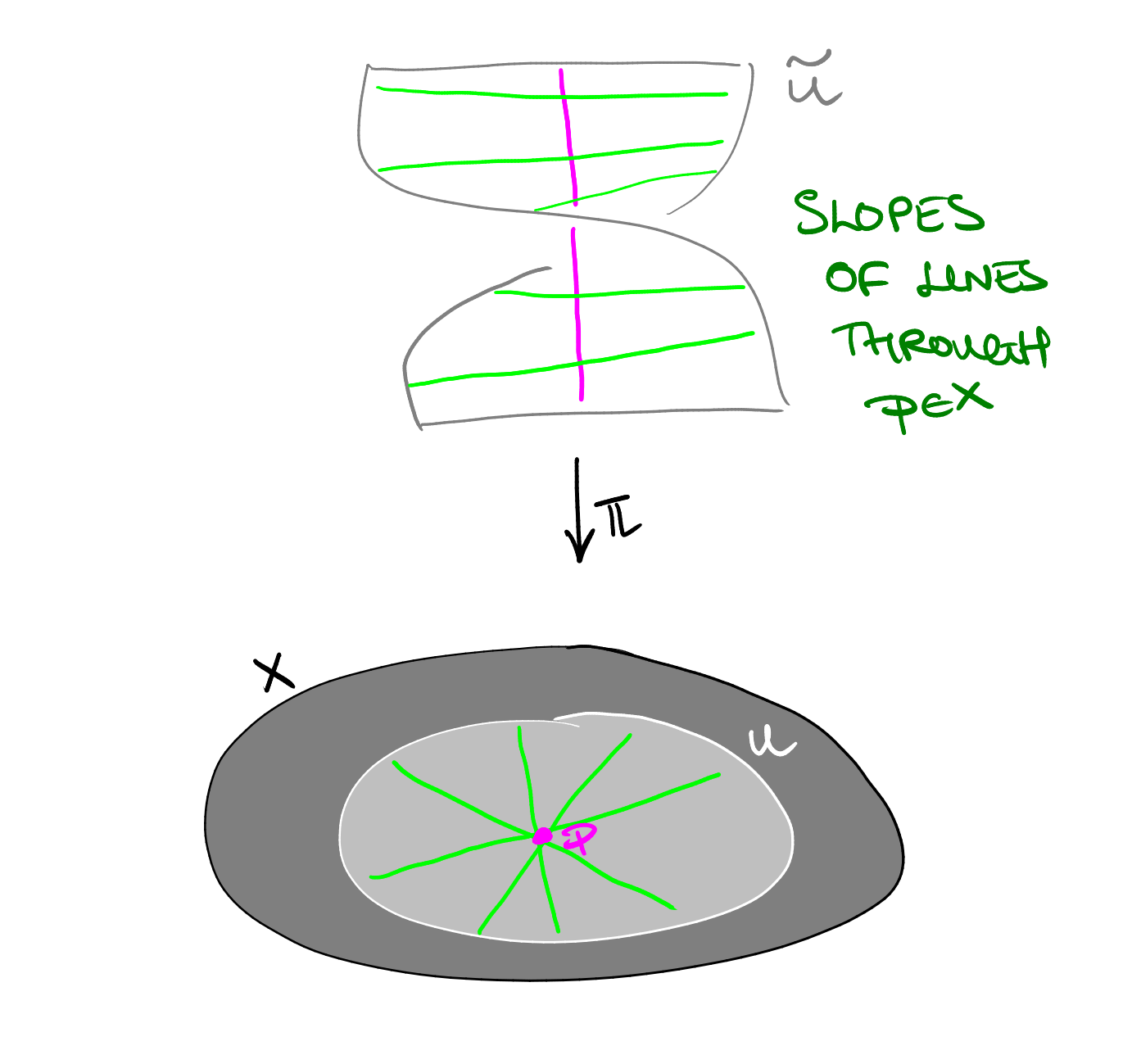
Remark 7.2.

The construction in Definition 7.1 works for smooth surfaces. More generally one does not need $X$ to be smooth – indeed this is often why one wants to blow-up, to resolve singularities. Even more generally we can define the blow-up of $X$ along an entire closed subscheme (not necessarily a point).

The following theorem follows easily from construction (except for uniqueness, which I leave as an exercise).

Theorem 7.3.

Let $X/k$ be a smooth projective surface and let $\pi :\tilde{X}\to X$ be the blow-up of $X$ at $p$ and let $V=X\setminus \{p\}$. Then

1. the morphism ${\pi |}_V$ is an isomorphism, and

2. the exceptional fibre $E={\pi }^{-1}(p)$ is isomorphic to ${\mathbb{P}}^1$.

Moreover $(\tilde{X},\pi )$ is unique up to isomorphism.

We start with some of the basic properties of the blow-up, after making a definition.

Definition 7.4.

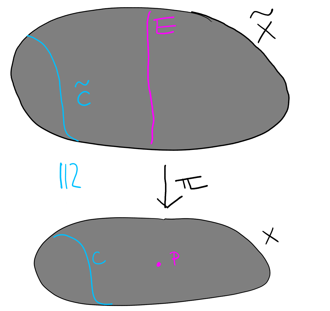
Let $\pi :\tilde{X}\to X$ be the blowup of $X$ at a point $p$. Let $C\subset X$ be an irreducible (reduced) curve, and define:

1. the strict transform of $C$ to be the Zariski closure $\tilde{C}=\overline{{\pi }^{-1}(C)}$ in $\tilde{X}$, and

2. the total transform of $C$ to be the pullback ${\pi }^{\ast }C\in \mathrm{Div}(\tilde{X})$.

We extend both constructions linearly to $\mathrm{Div}(X)$.

Figure 5. Different behaviours of the strict transform of a curve $C\subset X$ under blowup.

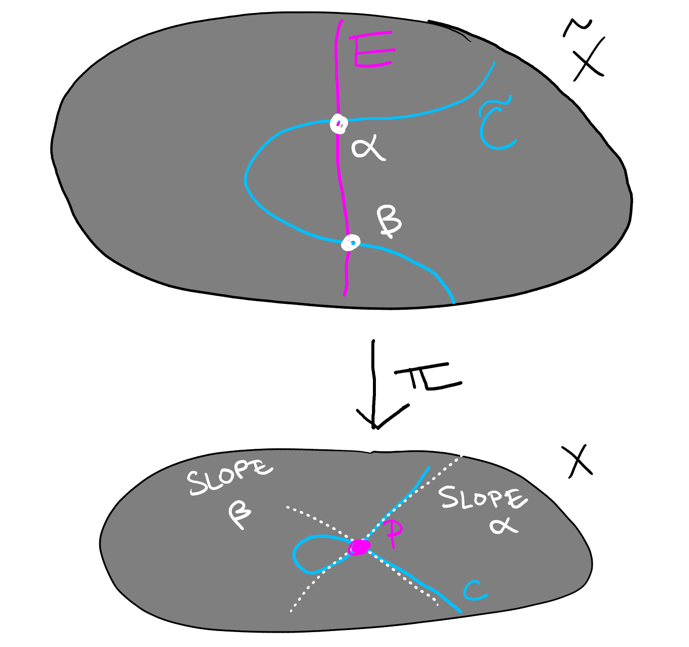
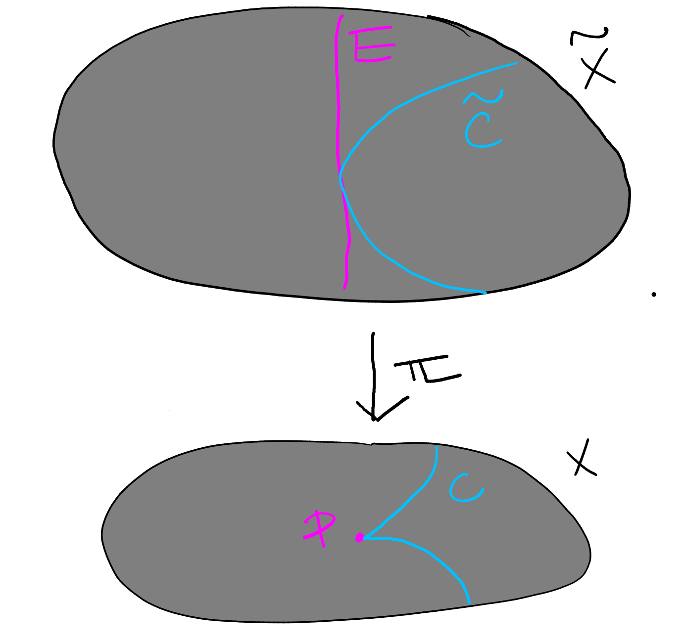
Lemma 7.5.

Let $C\subset X$ be a curve, and let $m\ge 0$ be the multiplicity with which $C$ passes through $p$, then ${\pi }^{\ast }C=\tilde{C}+mE$.

Proof.

The idea is to work locally to see what happens with the pullback. First, note that ${\pi }^{\ast }C=\tilde{C}+nE$ for some integer $n$. Continuing with the above notation, let $x,y\in {𝒪}_{X,p}$ be local coordinates at $p$. In a neighbourhood of $p$ we have an equation for $C$ given by, say, $f(x,y)=0$. Now take a power series expansion in the completed local ring ${\widehat{𝒪}}_{X,p}$

$$f(x,y)=f_m(x,y)+f_{m+1}(x,y)+\mathrm{\dots }$$

where each $f_i(x,y)$ is a homogeneous polynomial of degree $i$ in $x,y$. Consider the local coordinates $x$ and $t=T/S$ at the point $(p,\mathrm{\infty })$ on $\tilde{U}$ (with the notation of Definition 7.1). By definition we have $y=xt$. Now we compute

${\pi }^{\ast }f(x,y)$ $=f_m(x,tx)+f_{m+1}(x,tx)+\mathrm{\dots }$

$=x^m(f_m(1,t)+x{f}_{m+1}(1,t)+\mathrm{\dots })$

because each polynomial $f_i(x,y)$ is homogeneous of degree $i$. But we then visibly see that $n=m$. ∎

Proposition 7.6.

Let $\pi :\tilde{X}\to X$ be the blowup of $X$ at a point $p$ and let $E={\pi }^{-1}(p)$ be the exceptional divisor.

1. We have an isomorphism

   $\mathrm{Pic}(X)\times \mathbb{Z}$ $\stackrel{\sim }{⟶}\mathrm{Pic}(\tilde{X})$

   $(D,E)$ $⟼{\pi }^{\ast }D+nE.$

2. For any $D,D^{\prime }\in \mathrm{Div}(X)$ we have $({\pi }^{\ast }D\cdot {\pi }^{\ast }{D}^{\prime })=(D\cdot D^{\prime })$.

3. For any $D\in \mathrm{Div}(X)$ we have $({\pi }^{\ast }D\cdot E)=0$.

4. The self intersection $E^2=-1$.

5. A canonical divisor on the blow-up is given by $K_{\tilde{X}}={\pi }^{\ast }{K}_X+E$.

Proof.

The claims in (1)–(3) are clear when the support of $D$ and $D^{\prime }$ do not contain $p$. But these properties are invariant under replacing divisors by an element of their linear equivalence class. Applying the moving lemma (5.3) we are free to assume that the supports of $D$ and $D^{\prime }$ do not contain $p$.

For (4) let $C\subset X$ be a curve passing through $p$ with multiplicity $1$ (such a curve always exists because $X$ is smooth). Then by Lemma 7.5

${\pi }^{\ast }C\cdot E=(\tilde{C}+E)\cdot E=1+E^2$

so that by (3) one has $E^2=-1$.

Finally for (5) we argue as follows. Away from the exceptional divisor $E$ the zeroes and poles of a rational $2$-form $\omega \in {\mathrm{\Omega }}_{k(X)/k}^2$ are equal to that of its pullback ${\pi }^{\ast }\omega$. In particular $K_{\tilde{X}}\sim {\pi }^{\ast }{K}_X+nE$ for some integer $n$. Now $E\cong {\mathbb{P}}^1$ is a smooth curve of genus $0$, so by the genus formula and (3)

$2p_g(E)-2$ $=E\cdot (K_{\tilde{X}}+E)$

$=E\cdot ({\pi }^{\ast }{K}_X+(n+1)E)$

$=-(n+1)$

so that $n=1$. ∎

7.1. Castelnuovo’s contraction criterion

Proposition 7.6 says that if we blow-up a smooth surface at a point the exceptional divisor is a $(-1)$-curve, that is $E\cong {\mathbb{P}}^1$ and $E^2=-1$. There is a converse to this.

Theorem 7.7 (Castelnuovo’s contraction criterion).

Let $X/k$ be a smooth projective surface and let $E\subset X$ be a $(-1)$-curve. Then there exists a smooth projective surface $Y/k$ together with a morphism $\pi :X\to Y$ such that:

1. $\pi (E)=p$ is a point, and

2. $\pi$ is the blowup of $Y$ at $p$.

Vague sketch of the proof. Take some very ample divisor $H$ (a hyperplane section of some projective embedding $X\subset {\mathbb{P}}^n$) and choose a basis $x_0,\mathrm{\dots },x_n\in H^0(X,{𝒪}_X(H))$. Now suppose that $h^0(X,{𝒪}_X(H+mE))=h^0(X,{𝒪}_X(H))+1$ for some $m\ge 1$ – this is not always the case, but it’s way easier to sketch the proof. Now choose $y\in H^0(X,{𝒪}_X(H+mE))$ so that $x_0,\mathrm{\dots },x_n,y\in H^0(X,{𝒪}_X(H))$ is a basis. This gives a rational map

$\phi :$ $X⇢{\mathbb{P}}^{n+1}$

$P⟼(x_0(P):\mathrm{\dots }:x_n(P):y(P)).$

which is an embedding away from $E$ (since $x_0,\mathrm{\dots },x_n$ already gives a projective embedding of $X$). Since we chose $y\in H^0(X,{𝒪}_X(H+mE))$ so that $y\notin H^0(X,{𝒪}_X(H))$ it must be the case that $y$ has a pole along $E$. But if the functions $x_0,\mathrm{\dots },x_n$ have a pole at $P$ it occurs to a lesser degree than that of $y$. So for any point $P\in E$ we have $\phi (P)=(x_0(P):\mathrm{\dots }:x_n(P):y(P))=(0:\mathrm{\dots }:0:1)$. In this way $E$ is contracted to a point.

Subtleties: There are a bunch of subtleties here, and this is why the proof in [1, Theorem II.17] is much longer than this.

• To make sure that you can do this you should choose $H$ in such a way that $h^1(X,{𝒪}_X(H))=0$ (this can always be done by Serre vanishing). This way one can control $H^0(X,{𝒪}_X(H+mE))$ using the ideal sheaf exact sequence together with $H^0(X,{𝒪}_X(H))$ and ${𝒪}_E$ (and nice facts like ${𝒪}_E({E|}_E)\cong {𝒪}_{{\mathbb{P}}^1}({\mathrm{deg}E|}_E)={𝒪}_{{\mathbb{P}}^1}(E^2)={𝒪}_{{\mathbb{P}}^1}(-1)$).

• You may end up with way more $y$’s than just one (and if you don’t use them all you’ll get something singular) – this is a mild problem, it just requires some notation in order to define $\phi$.

• This just leaves the big issue of showing the image of $\phi$ is smooth. To get this you need to choose $m=(E\cdot H)$, though there is still a lot of work from here.

7.2. Elimination of indeterminacy

The following theorem shows that blowups are in a rigorous sense the “fundamental” birational transformations for smooth projective surfaces.

Theorem 7.8.

Let $\varphi :X⇢X^{\prime }$ be a birational map between smooth projective surfaces $X$ and $X^{\prime }$. Then there exists a smooth projective surface $\widehat{X}$ and a commutative diagram

such that the morphisms $f$ and $g$ are compositions of isomorphisms and blow-ups.

Proof.

Omitted, see [1, Corollary II.12]. ∎

8. Lines and $27=6+17+6$

We now have the tools to prove the famous 27 lines theorem (we do have them, but we won’t prove it completely). What we will prove is 8.7, which says that the blowup of ${\mathbb{P}}^2$ at $6$ points in general position is a smooth cubic surface containing exactly $27$ lines. This is a bit lame, since every smooth cubic surface is such a blowup, but we won’t prove it. Instead we settle for a rigorous “almost all”.

Theorem 8.1 (Cayley–Salmon, 1849).

Every almost all smooth cubic surfaces $X\subset {\mathbb{P}}^3$ contains exactly 27 lines.

The basic idea of the proof of this theorem (which is not the Cayley–Salmon proof) is to recognise $X$ as the blowup of ${\mathbb{P}}^2$ at $6$ points. The lines then come out of the blowup procedure. A slightly more general definition (which we will not use) is the following.

Definition 8.2.

A del Pezzo surface of degree $1\le d\le 8$ is a blowup of ${\mathbb{P}}^2$ at $9-d$ points in general position (i.e., no $3$ points are on a line and no $6$ are on a conic).

Lemma 8.3.

A del Pezzo surface of degree $3$ is isomorphic to a smooth cubic surface in ${\mathbb{P}}^3$.

Sketch proof. Let $p_1,\mathrm{\dots },p_6\in {\mathbb{P}}^2(k)$ be 6 points in general position, and let $\pi :Y\to {\mathbb{P}}^2$ be the blowup of ${\mathbb{P}}^1$ at $p_1,\mathrm{\dots },p_6$. Consider the vector space $S\subset k[x_0,x_1,x_2]$ of cubic polynomials which vanish on $p_1,\mathrm{\dots },p_6$ and note that ${dim}_{k}S=4$ (there are $10$ cubic monomials and $6$ linear conditions). Choose a $k$-basis $f_0,f_1,f_2,f_3\in S$ and let

$\phi :Y⇢{\mathbb{P}}^3$

be the rational map induced by the natural map ${\mathbb{P}}^2⇢{\mathbb{P}}^3$ given by our choice of basis. The Zariski closure of the image of $\phi$ is clearly a cubic surface.

Exercise 8.4 (Hard, see [1, Prop. 4.9]).

Check that $\phi$ is an isomorphism onto its image by checking that $\phi$ separated points and tangent directions. To do this on the exceptional divisors construct explicit polynomials in $S$ which pick out the slopes at the points $p_i$ (the parameters on $E_i$) by using lines and conics through the $p_i$.

Remark 8.5.

More generally than Lemma 8.3 a del Pezzo surface of degree $3\le d\le 8$ is isomorphic to a smooth surface of degree $d$ in ${\mathbb{P}}^d$. Here by degree I mean that you should intersect the surface $X\subset {\mathbb{P}}^d$ with two general hyperplanes $H,H^{\prime }$ and then count $\mathrm{\#}(X\cap H\cap H^{\prime })$.

Lemma 8.6.

Let $X$ be a smooth cubic surface and let $L\subset X$ be a smooth irreducible curve, then $L^2=-1$ if and only if $L$ is a line.

Proof.

By the adjunction formula Theorem 5.9 we have $K_X=-{H|}_X$ for any hyperplane $H\subset {\mathbb{P}}^3$. In particular we have $K_X\cdot L=-({H|}_X\cdot L)$. Choosing $H$ so that $L\not\subset H$ and counting intersections we see that $K_X\cdot L=-1$ if and only if $L$ is a line. Thus by the genus formula Theorem 6.8 we have $K_X\cdot L=L^2=-1$ if and only if $L$ is a line. ∎

Proposition 8.7.

Let $X\subset {\mathbb{P}}^3$ be a cubic surface which is isomorphic to the blowup of ${\mathbb{P}}^2$ at 6 points $p_1,\mathrm{\dots },p_6$ in general position. Then the lines on $X$ are exactly:

1. the exceptional divisors $E_1,\mathrm{\dots },E_6$ above the points $p_1,\mathrm{\dots },p_6$,

2. the strict transforms ${\tilde{M}}_{ij}$ where $M_{ij}\subset {\mathbb{P}}^2$ is the line through $p_i$ and $p_j$, and

3. the strict transforms ${\tilde{Q}}_i$ where $Q_i\subset {\mathbb{P}}^2$ is the conic through each $p_j\ne p_i$.

In particular $X$ contains $6+\left(\genfrac{}{}{0pt}{}{6}{2}\right)+6=6+15+6=27$ lines.

Proof.

By Proposition 7.6 we have $\mathrm{Pic}(X)\cong \mathbb{Z}\tilde{C}{⨁}_i\mathbb{Z}{E}_i$ and $K_X\sim -3\tilde{C}+{\sum }_{i=1}^6{E}_i$ for any line $C\subset {\mathbb{P}}^2$ not containing $p_i$ for each $i=1,\mathrm{\dots },6$.

Let $L\subset X$ be a line and suppose that $L\ne E_i$ for any $i$. By the relation on Picard groups we may write $L\sim m\tilde{C}-{\sum }_{i=1}^6{m}_i{E}_i$ and note that by Lemma 8.6 we have

(8.1) $$1=-(K_X\cdot L)=\left(3\tilde{C}-\sum _{i=1}^6{E}_i\right)\cdot \left(m\tilde{C}-\sum _{i=1}^6{m}_i{E}_i\right).$$

Since the line $C$ was chosen so that $p_i\notin C$ we have $(\tilde{C}\cdot E_i)=0$ for each $i$ and ${\tilde{C}}^2=C^2=1$. Noting also that $(E_i\cdot E_j)=0$ for each $i\ne j$, by (8.1) we have

(8.2) $$3m-\sum _{i=1}^6{m}_i=1.$$

Now, each exceptional curve $E_i$ is a line (by Lemma 8.6) and $L$ is a line (by assumption) we have $m_i=(L\cdot E_i)=\mathrm{\#}(L\cap E_i)\in \{0,1\}$. Therefore the allowable combinations in (8.2) are:

• there exist $i\ne j$ such that $m_i=m_j=1$ and $m_{\mathrm{\ell }}=0$ for each $\mathrm{\ell }\ne i,j$, and

• there exists $i$ such that $m_i=0$ and $m_j=0$ for each $j\ne i$.

In the first case we have $L={\tilde{M}}_{i,j}$ and in the second we have $L={\tilde{Q}}_i$. ∎

8.1. Almost all cubic surfaces are the blowup of ${\mathbb{P}}^2$ at $6$ points

Here is a cheap trick to show that almost all cubic surfaces are the blowup of ${\mathbb{P}}^2$ at $6$ points in general position. This comes from [2, V.4]. For the actual result see [1, Theorem IV.13].

Proposition 8.8.

Every almost all cubic surfaces are isomorphic to the blowup of ${\mathbb{P}}^2$ at $6$ points in general position.

Proof.

The argument is via moduli. We showed in Lemma 8.3 that every such surface $X$ is a smooth cubic surface, so we have a finite-to-one map

$$({\mathrm{Sym}}^6({\mathbb{P}}^2)\setminus \left\{\text{points not in general position}\right\})/{\mathrm{PGL}}_3\to \left\{\text{smooth cubic surfaces}\right\}/\sim .$$

On the other hand we have that

$$(\{\text{cubic polynomials }f\in k[x_0,x_1,x_2,x_3]\}\setminus \{f:𝕍(f)\text{ is singular}\})/{\mathrm{PGL}}_4\leftrightarrow \left\{\text{smooth cubic surfaces}\right\}/\sim .$$

Note that the conditions “not in general position” and “defining a singular surface” are Zariski closed on the ambient space. Therefore, to show that almost all cubic surfaces arise it suffices to show that the dimensions of the objects on the left hand side are the same.

To see this note that the dimension of ${\mathrm{Sym}}^6({\mathbb{P}}^2)/{\mathrm{PGL}}_3$ is $12-8=4$. There are $\left(\genfrac{}{}{0pt}{}{4+3-1}{4-1}\right)=20$ cubic monomials in $4$ variables, so the dimension of the space of smooth cubic surfaces up to the action of ${\mathrm{PGL}}_4$ is $20-16=4$, as required. ∎

9. Cohomological invariants

We now introduce a bunch of useful cohomological invariants of smooth projective varieties.

Definition 9.1.

Let $X/k$ be a smooth projective algebraic variety of dimension $n$. We define:

• the geometric genus

  $$p_g(X)=h^0(X,{\omega }_X)$$

• the Euler characteristic of the structure sheaf

  $$\chi ({𝒪}_X)$$

• the arithmetic genus

  $$p_a(X)={(-1)}^n(\chi ({𝒪}_X)-1)$$

• the $n^{\text{<em class="ltx\_emph" style="font-size:70\%;">th</em>}}$-plurigenus for $n\ge 1$

  $$P_n(X)=h^0(X,{\omega }_X^{\otimes n})$$

• if $X$ is a surface we define the irregularity

  $$q(X)=h^1(X,{𝒪}_X)=p_g(X)-p_a(X)$$

By Hodge theory one has $q(X)=h^0(X,{\mathrm{\Omega }}_X)$ (you may see $h^{1,0}=h^{0,1}$).

Proposition 9.2.

The integers $p_g(X)$, $\chi ({𝒪}_X)$, $p_a(X)$, $P_n(X)$, and $q(X)$ are birational invariants of smooth projective surfaces.

Proof idea.

The basic idea for $p_g$ (and $P_n$) is to use two things:

1. Birational maps $X⇢Y$ between proper (e.g., projective) varieties can be extended to a morphism on open subsets $U\to V$ where $X\setminus U$ has co-dimension $2$ in $X$.

2. With the notation in (1) we have $h^0(X,{\omega }_X)=h^0(U,{\omega }_U)$.

For $q(X)$ one proves things similarly using the equality $q(X)=h^0(X,{\mathrm{\Omega }}_X)$ and an argument like (2) (see [1, Prop. III.20]). ∎

9.1. Examples of surfaces

We start with the “most obvious” example – a product of smooth curves.

Theorem 9.3.

Let $C_1$ and $C_2$ be smooth curves of genera $g_1$ and $g_2$ respectively. If $X=C_1\times C_2$ we have

$p_g(X)$ $=g_1{g}_2,$

$\chi ({𝒪}_X)$ $=(1-g_1)(1-g_2),$

$q(X)$ $=g_1+g_2,$

$p_a(X)$ $=g_1{g}_2-(g_1+g_2).$

Proof.

We first make use of the Künneth formula ([8, Lemma 0BED]) which in our situation says that

$$H^n(X,{𝒪}_X)=\underset{p+q=n}{⨁}{H}^p(C_1,{𝒪}_{C_1})\otimes H^q(C_2,{𝒪}_{C_2}).$$

In particular we have

$h^0(X,{𝒪}_X)$ $=1$

$h^1(X,{𝒪}_X)$ $=h^1(C_1,{𝒪}_{C_1})+h^1(C_1,{𝒪}_{C_2})$

$=g_1+g_2$

$h^2(X,{𝒪}_X)$ $=h^1(C_1,{𝒪}_{C_1})h^1(C_1,{𝒪}_{C_2})$

$=g_1{g}_2.$

But then $p_g(X)=h^0(X,{\omega }_X)=h^2(X,{𝒪}_X)=g_1{g}_2$ (the second equality being Serre duality), and similarly for the other cases. ∎

Corollary 9.4.

There are infinitely many non-birational algebraic surfaces.

Proof.

Immediate from 9.2 and Theorem 9.3. ∎

Theorem 9.5.

Let $X\subset {\mathbb{P}}^3$ be a smooth projective surface of degree $d$, then

$p_g(X)$ $={\displaystyle \frac{1}{6}}(d-1)(d-2)(d-3),$

$q(X)$ $=0.$

Proof.

We have the ideal sheaf exact sequence

$$0\to {𝒪}_{{\mathbb{P}}^3}(-d)\to {𝒪}_{{\mathbb{P}}^3}\to {\iota }_{\ast }{𝒪}_X\to 0.$$

Thus $\chi ({𝒪}_X)=\chi ({𝒪}_{{\mathbb{P}}^3})-\chi ({𝒪}_{{\mathbb{P}}^3}(-d))$. Here is a super useful fact.

Lemma 9.6 (Hilbert polynomial).

Let $X\subset {\mathbb{P}}^n$ be a smooth projective variety, then there exists a polynomial $h_X(t)\in \mathbb{Z}[t]$ such that $h_X(m)=\chi ({𝒪}_X(m))$ for all $m\in \mathbb{Z}$.

Now by Serre vanishing, for all $m\gg 0$ we have

$\chi ({𝒪}_{{\mathbb{P}}^n}(m))$ $=h^0({\mathbb{P}}^n,{𝒪}_{{\mathbb{P}}^n}(m))$

$=\mathrm{\#}\{\text{monomials of degree }m\text{ in }n+1\text{ variables}\}$

$=\left({\displaystyle \genfrac{}{}{0pt}{}{n+m}{n}}\right)$

$=\frac{1}{n!}(m+n)(m+n-1)\mathrm{\dots }(m+1).$

But note that this equality hold for infinitely many integers $m$, so that for ${\mathbb{P}}^3$ the Hilbert polynomial is

$$h_{{\mathbb{P}}^3}(t)=\frac{1}{6}(t+3)(t+2)(t+1).$$

In particular, we have $\chi ({𝒪}_X)=h_{{\mathbb{P}}^3}(0)-h_{{\mathbb{P}}^3}(-d)=1+\frac{1}{6}(d-1)(d-2)(d-3)$. Thus $p_a(X)=\frac{1}{6}(d-1)(d-2)(d-3)$ as required. It remains to show that $q(X)=0$, which we will not do. It follows from the fact that $q(X)=h^0(X,{\mathrm{\Omega }}_X)=\frac{1}{2}{b}_1(X)$ (Betti number) together with the fact that a projective hypersurface is simply connected (Lefshetz hyperplanes). ∎

Remark 9.7.

This is what you would naïvely expect, because we already know that degree $1$, $2$, and $3$ surfaces are rational (hence the $(d-1)(d-2)(d-3)$). One should compare with the genus-degree formula for curves (Proposition 6.10).

9.2. Kodaira dimension

Our final invariant is the Kodaira dimension, which measures “how well we can use $K_X$ to embed $X$”.

For some $m\ge 1$ suppose that $h^0(X,{𝒪}_X(m{K}_X))\ne 0$ and choose a basis of rational functions $x_0,\mathrm{\dots },x_n\in H^0(X,{𝒪}_X(m{K}_X))$. Define a rational map

${\phi }_m:X$ $⇢{\mathbb{P}}^n$

$P$ $⟼[x_0(P):\mathrm{\dots }:x_n(P)].$

Definition 9.8.

If for some $m\ge 1$ we have $h^0(X,{𝒪}_X(m{K}_X))\ne 0$, we define that Kodaira dimension of $X$ to be

$$\kappa (X)=\underset{m\ge 1}{\max }(dim\overline{{\phi }_m(X)}).$$

If $h^0(X,{𝒪}_X(m{K}_X))=0$ for all $m\ge 1$ we define $\kappa (X)=-\mathrm{\infty }$.

Some authors prefer $-1$ rather than $-\mathrm{\infty }$.

Example 9.9.

1. Take $X={\mathbb{P}}^n$ so that $K_X\sim -(n+1)H$ where $H$ is any hyperplane. Then

   $$h^0({\mathbb{P}}^n,{𝒪}_{{\mathbb{P}}^n}(m{K}_{{\mathbb{P}}^n}))=h^0({\mathbb{P}}^n,{𝒪}_{{\mathbb{P}}^n}(-m(n+1)))=0$$

   for all $m\ge 1$. So, as per the definition, we have $\kappa ({\mathbb{P}}^n)=-\mathrm{\infty }$.

2. Take $X$ to be an elliptic curve. Then $K_X\sim 0$ and therefore

   $$h^0(X,{𝒪}_X(m{K}_X))=h^0(X,{𝒪}_X)=1$$

   for all $m\ge 1$. Thus the map ${\phi }_m$ takes $X$ to a point and $\kappa (X)=0$.

3. Take $X\subset {\mathbb{P}}^3$ to be a smooth quartic surface. Then by the adjunction formula $K_X\sim 0$ and as above $\kappa (X)=0$. This clearly generalises to a smooth degree $n+1$ hypersurface in ${\mathbb{P}}^n$.

Exercise 9.10.

1. Show that if $X$ is a smooth projective curve of genus $\ge 2$ then $\kappa (X)=1$.

2. Show that if $X$ is a smooth surface of degree $5$ then $\kappa (X)=2$.

3. Show that if $X$ is a smooth surface of degree $\ge 5$ then $\kappa (X)=2$.

9.3. The rationality criterion

If $X/k$ is a smooth projective curve, there is a cohomological criterion which allows us to tell whether or not $X$ is birational (isomorphic) to ${\mathbb{P}}^1$.

Lemma 9.11.

A smooth projective curve $X/k$ is birational to ${\mathbb{P}}^1$ if and only if $p_g(X)=0$.

It is natural to wonder if having the same geometric genus as ${\mathbb{P}}^2$ is enough to be a rational surface. Of course, this is false – by Theorem 9.3 if $C$ has genus $\ge 1$ then the ruled surface $X={\mathbb{P}}^1\times C$ has $p_g(X)=0$ and $q(X)\ge 1$. Now we have $h^0$, $h^1$, and $h^2$ covered, one might conjecture that $p_g(X)=q(X)=0$ is sufficient to show that $X$ is birational to ${\mathbb{P}}^2$. Maybe surprisingly this is false (e.g., Enriques surfaces are not rational), however there is a cohomological criterion for rationality.

Theorem 9.12 (Castelnuovo’s rationality criterion).

A smooth projective surface $X/k$ with $P_2(X)=q(X)=0$ is rational.

I will not give a proof of this theorem (see [1, V.1]) however the following is my crude understanding of the proof. One of the central ingredients is the following fact.

Fact.

Let $X$ be as in the theorem, and suppose that $C\subset X$ is a rational curve with $C^2>0$. Then $X$ is rational.

One should maybe think of $C^2>0$ saying that the curve $C$ can move among effective divisors in its linear equivalence class. The fact is then saying that if such a curve exists, then the cohomological facts are enough to sweep $C$ all across $X$ (hence giving a ruling). One then has the job of going into the weeds to find such a curve.

10. Enriques–Kodaira classification

A very sketchy description of the classification of algebraic surfaces follows.

Definition 10.1.

Let $X/k$ be a smooth projective surface then:

1. $X$ is said to be rational if it is birational to ${\mathbb{P}}^2$, and

2. $X$ is said to be ruled if it is birational to ${\mathbb{P}}^1\times C$ where $C$ is a curve.

Exercise 10.2.

Show that if $X/k$ is a ruled surface, then $\kappa (X)=-\mathrm{\infty }$.

To classify surfaces, it is extremely useful to know that we only need to do biregular geometry (i.e., up to isomorphisms) as opposed to birational geometry (i.e., up to birational maps). To ensure this, we wish to work with a unique model in each birational equivalence class. This is ever-so-slightly too much to hope for, but if $X$ is not ruled we can get this, as we now see. A proof can be found in [1, Prop. 2.16 and Theorem V.19].

Definition 10.3.

We say that a smooth, projective surface $X/k$ is minimal if it contains no $(-1)$-curves. Equivalently, $X$ is minimal if and only if every birational map $X\to X^{\prime }$ is an isomorphism.

Theorem 10.4 (Existence and uniqueness of minimal models).

If $X/k$ is a smooth, projective surface then there exists a dominant (i.e., surjective on $k$-points) birational morphism $\pi :X\to X^{\prime }$ where $X^{\prime }$ is minimal.

Moreover, if $X$ is not a ruled surface, then $X^{\prime }$ is unique and is obtained from $X$ by blowing down a finite number of $(-1)$-curves.

For the proof, just blow-down all the $(-1)$-curves (of course, there is more to show — it terminates, it terminates at something unique, etc).

10.1. $\kappa (X)=-\mathrm{\infty }$

It is a theorem of Enriques that this case is entirely covered by ruled surfaces.

Theorem 10.5 (Enriques’ Theorem).

Let $X/k$ be a smooth projective surface. Then the following are equivalent:

1. $\kappa (X)=-\mathrm{\infty }$,

2. $P_n(X)=0$ for all $n\ge 1$,

3. $X$ is a ruled surface.

Note that the (2)$⟹$(3) case of Theorem 10.5 is closely related to Castelnuovo’s rationality criterion (a ruled surface with $q(X)=0$ is rational).

10.2. $\kappa (X)=0$

This case is really the guts of the classification. First we define some surfaces which we have been playing with a lot.

Definition 10.6.

Let $X/k$ be a smooth projective (algebraic) surface. We say that:

1. $X$ is is an (algebraic) K3 surface if $K_X\sim 0$ and $q(X)=0$,

2. $X$ is an Enriques surface if $K_X\sim ̸0$, $2K_X\sim 0$, and $p_g(X)=q(X)=0$,

3. $X$ is a bi-elliptic surface if $X\cong (E\times E^{\prime })/G$ where $E$ and $E^{\prime }$ are elliptic curves and $G\cong \mathbb{Z}/m\mathbb{Z}$ is a cyclic group acting by translations on $E$ and not by translations on $E^{\prime }$.

4. $X$ is an abelian surface if $X(ℂ)\cong {ℂ}^2/\mathrm{\Lambda }$ (as complex manifolds) for some full-rank lattice $\mathrm{\Lambda }\subset {ℂ}^2$.

Remark 10.7.

1. It may not be immediately obvious that Enriques surfaces actually exist.

2. Note that the condition on a bi-elliptic surface means that $m\in \{2,3,4,6\}$ and in the latter $3$ cases $j(E^{\prime })\in \{0,1728\}$.

3. An abelian surface can also be defined as an abelian variety of dimension $2$. An abelian variety is a projective, algebraic group variety (i.e., a projective variety $A/k$ equipped with an identity $O\in A$ and “inversion” and “multiplication” morphisms $i:A\to A$ and $m:A\times A\to A$ doing the obvious things).

We can now state the Enriques–Kodaira classification in the Kodaira dimension $0$ case.

Theorem 10.8 (Enriques–Kodaira).

Let $X/k$ be a minimal smooth projective algebraic surface with $\kappa (X)=0$. Then $X$ is either:

1. an algebraic K3 surface ($p_g(X)=1$ and $q(X)=0$),

2. an Enriques surface ($p_g(X)=0$ and $q(X)=0$),

3. a bi-elliptic surface ($p_g(X)=0$ and $q(X)=1$), or

4. an abelian surface ($p_g(X)=1$ and $q(X)=2$).

10.2.1. Examples of K3 surfaces

We have seen many K3 surfaces so far. The following exercise lists some of them.

Exercise 10.9.

Show that each of the following surfaces is a K3 surface.

1. A smooth quartic surface.

2. A complete intersection of a quadric and cubic in ${\mathbb{P}}^4$.

3. A complete intersection of $3$ quadrics in ${\mathbb{P}}^5$.

4. A double cover of ${\mathbb{P}}^2$ ramified over a smooth curve of degree $6$. (Hint: use that if $\pi :X\to Y$ is a finite morphism between smooth projective varieties $X$ and $Y$ then $K_X\sim {\pi }^{\ast }{K}_Y+R$ where $R$ is the ramification locus of $\pi$.)

10.2.2. Examples of Enriques surfaces

For Enriques surfaces, the construction is somewhat more involved, but there is a very useful proposition (see [1, Prop. VIII.17]).

Proposition 10.10.

Let $Y/k$ be a K3 surface equipped with an involution $\tau$ (i.e., a map $\tau :Y\to Y$ for which ${\tau }^2=\mathrm{id}$). Then the quotient $X=Y/\tau$ is a smooth projective algebraic surface and an Enriques surface. Moreover, every Enriques surface arises in this way.

Sketch proof.

Smoothness of the quotient follows since the action of $\tau$ has no “isolated” fixed points (indeed, it has no fixed points at all…).

Fact.

If $\pi :X\to Y$ is a finite morphism between smooth projective varieties $X$ and $Y$ then $K_X\sim {\pi }^{\ast }{K}_Y+R$ where $R$ is the ramification locus of $\pi$.

In our case, the fact says that $K_X\sim {\pi }^{\ast }{K}_Y$. For any divisor $D$ on $Y$ we have ${\pi }_{\ast }{\pi }^{\ast }D=(\mathrm{deg}\pi )D$. Thus ${\pi }_{\ast }{\pi }^{\ast }{K}_Y=2K_Y$ and noting that $K_X\sim 0$ (since $X$ is a K3 surface) we have $2K_Y=0$, as required. Now, since $\pi :X\to Y$ is étale we have $\chi ({𝒪}_X)=(\mathrm{deg}\pi )\chi ({𝒪}_Y)$. Because $X$ is a K3 surface $\chi ({𝒪}_X)=2$ and thus $\chi ({𝒪}_Y)=1$. In particular we must have $p_g(Y)=q(Y)=0$, as required.

The idea for the converse is the “cyclic covering trick” which says that those $ℒ\in \mathrm{Pic}(Y)$ with ${ℒ}^{\otimes 2}\cong {𝒪}_Y$ correspond exactly to étale double covers $X\to Y$. ∎

10.2.3. Examples of abelian surfaces

There are only two ways to build an abelian surface. The first is to take a product of elliptic curves $E\times E^{\prime }$ (it should be clear that this satisfies the definition). The second is a more involved construction called the Jacobian.

Proposition 10.11.

Let $C/ℂ$ be a smooth projective curve of genus $g$. Then there exists an algebraic variety $J_C/ℂ$ of dimension $g$ such that we have an isomorphism $J_C(ℂ)\cong H^0{(C,{\mathrm{\Omega }}_C^1)}^{\vee }/H_1(C,\mathbb{Z})$ as complex manifolds (and $J_C(ℂ)\cong {\mathrm{Pic}}^0(C)$ as groups). We call $J_C$ the Jacobian of $C$.

By Proposition 10.11 the Jacobian $J_C$ of a genus $2$ curve is an abelian surface. One needs to work harder to show that all abelian surfaces are isomorphic to either a product of elliptic curves or a Jacobian.

Exercise 10.12.

Let $A/k$ be an abelian surface and let $\iota :A\to A$ be the inversion map.

1. Show that the $\iota$ has exactly $16$ fixed points and deduce that the quotient $X=A/\iota$ has $16$-singular points.

2. Show that there exists a surface $\tilde{X}\to X$ which is non-singular and the exceptional divisor above each of the $16$ singular points is a $(-2)$-curve (i.e., a smooth rational curve with $C^2=-2$). (Hint: extend the action of $\iota$ to the blowup of $A$ at its $2$-torsion points.)

3. Show that $\tilde{X}$ is a K3 surface.

4. Let $P$ be a $2$-torsion point on $A$ and let ${\tau }_P:A\to A$ be the map $Q\mapsto Q+P$. Show that ${\tau }_P$ induces a morphism on $X$ (and thus on $\tilde{X}$). Find out what you can about $\tilde{X}/{\tau }_P$.

10.3. $\kappa (X)=1$

We call any surface $X/k$ of Kodaira dimension $1$ a properly elliptic surface (or elliptic surface of Kodaira dimension $1$). The reason for this will be explained.

Exercise 10.13.

Show that if $C$ is a curve of genus $\ge 2$ then the surface $E\times C$ is a properly elliptic surface.

Definition 10.14.

Let $C$ be a smooth projective curve. We say that a morphism $f:X\to C$ is an elliptic fibration if the generic fibre of $f$ is a smooth curve of genus $1$.

Figure 6. An elliptic fibration.

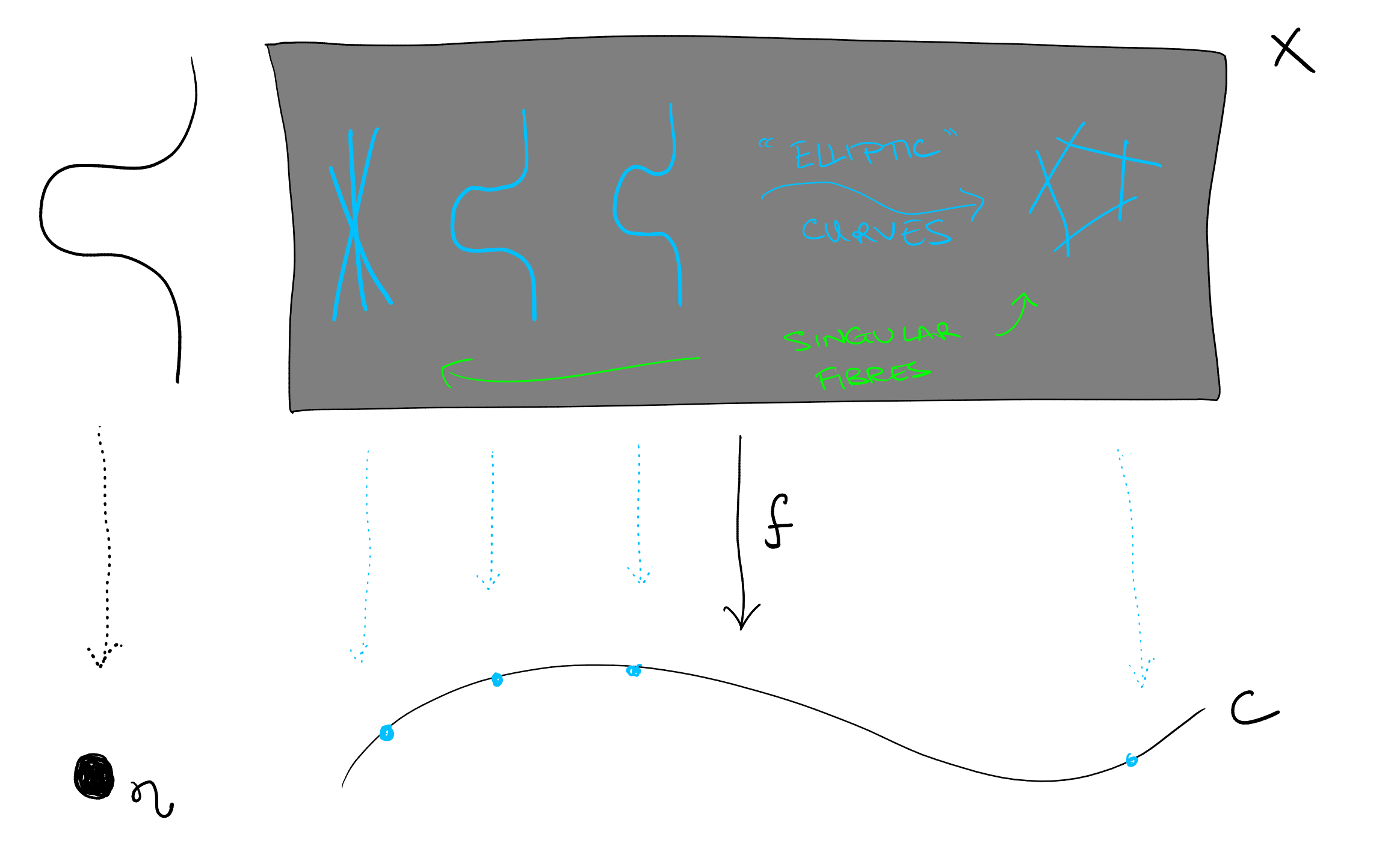
Remark 10.15.

Note that the above definition of an elliptic fibration does not require that there exists a $k(C)$-point on the generic fibre of $f$. Some authors might therefore be inclined to call the above a genus $1$ fibration and declare it to be elliptic if there exists a section $C\to X$ of $f$.

Theorem 10.16.

Let $X/k$ be a smooth projective surface with $\kappa (X)=1$. Then there exists a curve $C/k$ and an elliptic fibration $f:X\to C$.

Proof idea.

A complete proof is given in [1, IX].

From the definition of Kodaira dimension we know that there exists an integer $m\ge 1$ such that the (Zariski closure of the) image of the rational map ${\phi }_m:X⇢{\mathbb{P}}^n$ is a curve $B$ (here ${\phi }_m$ as defined in Section 9.2).

Assumption: ${\phi }_m$ is a morphism. (This can be avoided by breaking up the “fixed” and “mobile” parts of the linear system $|m{K}_X|$ see [1, IX].)

One might hope that ${\phi }_m$ is the elliptic fibration we are looking for, but the fibres can be disconnected. Fortunately there is “Stein factorisation” which says there exists a curve $C/k$ and a factorisation $X\to C\to B$ where the first morphism has connected fibres (call it $f$). To conclude we first need a standard lemma.

Lemma 10.17.

Let $f:X\to C$ be a morphism ($X$ a smooth projective surface and $C$ a smooth projective curve). If $F$ is a fibre of $f$, then $F^2=0$.

Proof.

Let $P\in C(k)$ be so that $F=f^{\ast }(P)$. By the moving lemma 5.3 there exists a divisor $D\in \mathrm{Div}(C)$ so that $D\sim P$ and the support of $D$ is disjoint from $P$. Then $F\sim f^{\ast }(D)$ and therefore $F^2=F\cdot f^{\ast }(D)=0$ (the fibre above $Q$ does not meet $F$ for any point $Q\ne P$). ∎

Figure 7. Illustration of the proof of Lemma 10.17.

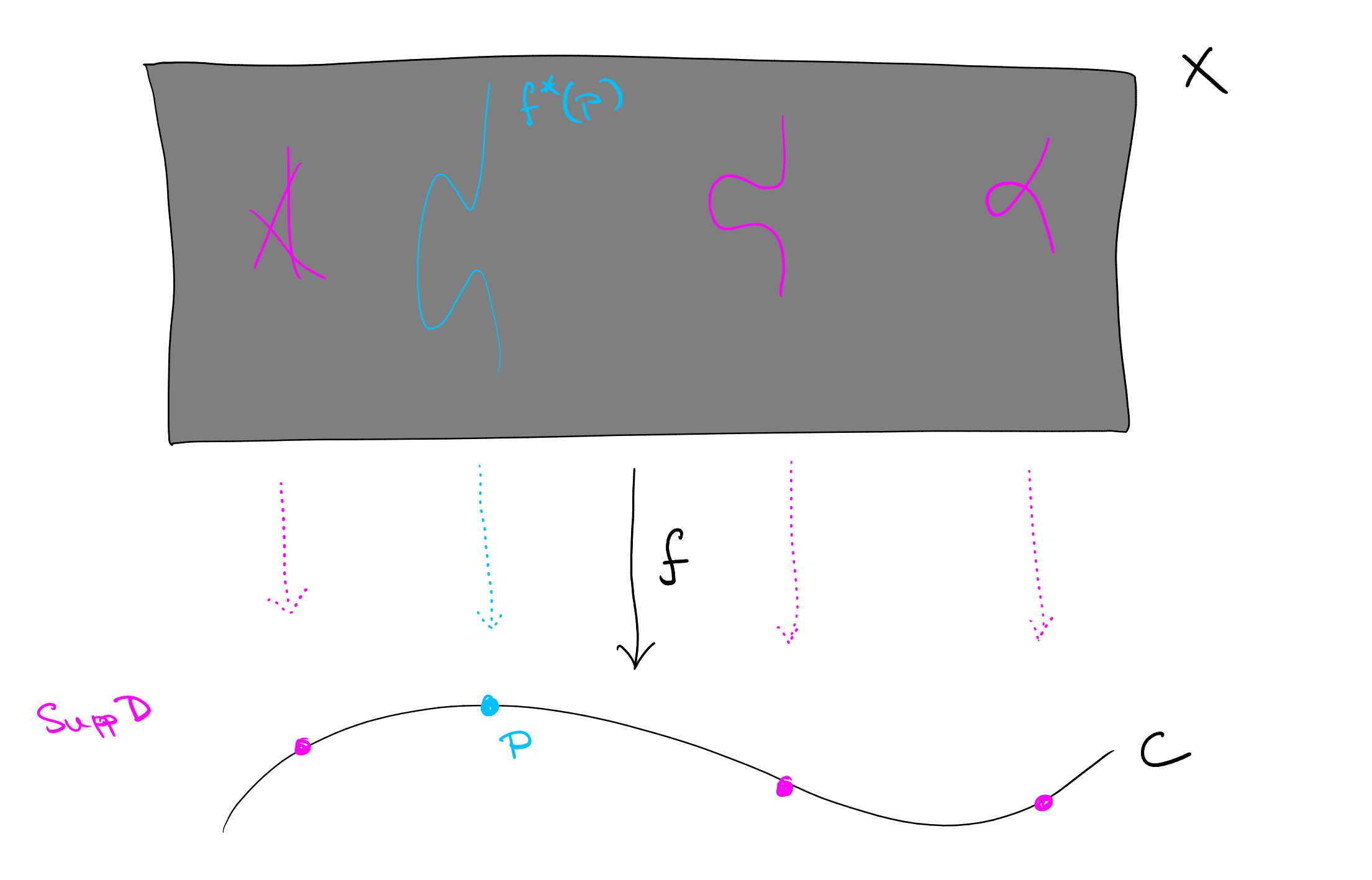
The final ingredient is the following useful proposition.

Proposition 10.18 ([1, Lemma IX.1]).

Suppose that $X$ is a smooth projective surface which is not ruled. Then

1. if $K_X^2>0$ then $X$ is of general type (i.e., $\kappa (X)=2$), and

2. if $X$ is minimal and not of general type then $K_X^2=0$.

Now, let $F$ be a general fibre of $X$ (i.e., if it is singular, re-choose it). By construction we have $F\sim m{K}_X$ (without our assumption that ${\phi }_m$ is a morphism, as is the case in in [1, IX], one has $F\sim M$ where $M$ is the “mobile part” of $m{K}_X$). By the genus formula (Theorem 6.8) we have

$2-2p_g(F)$ $=F\cdot (K_X+F)$

$=m(m+1)K_X^2$

$=0$

by Proposition 10.18(2) (and the assumption that $X$ is minimal). The conclusion follows. ∎

Exercise 10.19.

Construct a rational elliptic surface, an elliptic K3 surface, and a properly elliptic surface.

Exercise 10.20 (Hard?).

Let $A,B\in k[S,T]$ be homogeneous polynomials of degree $4n$ and $6n$ respectively. Consider the affine surface in $Y\subset {𝔸}^3$ given by

$$Y:y^2=x^3+A(t,1)x+B(t,1).$$

Suppose that $\mathrm{\Delta }=-16(16A^3+27B^2)\ne 0$. Let $X$ be a smooth projective surface birational to $Y$.

1. Show that $X$ admits an elliptic fibration $X\to {\mathbb{P}}^1$.

2. Suppose that $\mathrm{\Delta }$ is ${12}^{\text{th}}$-power free. Show that $X$ is:

   1. a rational surface if $n=1$,

   2. a (blown-up) K3 surface if $n=2$, and

   3. a properly elliptic surface if $n\ge 3$.

10.4. $\kappa (X)=2$

We simply define any surface with $\kappa (X)=2$ to be of general type. Examples are given in Exercise 9.10. At least we know the following.

Proposition 10.21 ([1, Lemma IX.1]).

Suppose that $X$ is a smooth projective surface which is not ruled. If $K_X^2>0$ then $X$ is of general type.

10.5. A table

The following table represents the Enriques–Kodaira classification, as described above.

$\kappa (X)$	$p_g(X)$	$q(X)$	Name
$-\mathrm{\infty }$	$0$	$0$	Rational
$-\mathrm{\infty }$	$0$	$\ge 1$	Ruled (not rational)
$0$	$1$	$0$	K3
$0$	$0$	$0$	Enriques
$0$	$0$	$1$	Bi-elliptic
$0$	$1$	$2$	Abelian
$1$	$\ge 0$	$\ge 0$	Properly elliptic
$2$	$\ge 0$	$\ge 0$	General type

Table 1. The Enriques–Kodaira classification

10.6. A very brief note on the proof

I will conclude with the briefest of notes on how one proves the Enriques–Kodaira classification (in particular Theorems 10.5 and 10.8). As you can may notice, much of the work lies in the Kodaira dimension $0$ case. Unfortunately, the morphism provided by the definition of Kodaira dimension does not carry nearly as much information as it does in the $\kappa (X)=1$ case. One instead needs an object associated to a different cohomological invariant. A central tool is the Albanese variety.

Definition 10.22.

Let $X/k$ be a smooth projective variety. The Albanese variety of $X$ is a pair $(\mathrm{Alb}X,\alpha )$ where $\mathrm{Alb}X$ is an abelian variety and $\alpha :X\to \mathrm{Alb}X$ is a morphism with the property that for any abelian variety $T/k$ and morphism $\varphi :X\to T$, there exists a unique factorisation

The Albanese generalises the Jacobian of a curve (which plays a crucial role in the theory of curves). Importantly, the Albanese exists.

Theorem 10.23 ([1, Theorem V.13]).

Let $X/k$ be a smooth projective variety. The Albanese variety of $X$ exists and the morphism $\alpha :X\to \mathrm{Alb}X$ is unique up to translation on the target.

A crucial property of the Albanese is that the morphism $\alpha$ induces an isomorphism ${\alpha }^{\ast }:H^0(\mathrm{Alb}X,{\mathrm{\Omega }}_{\mathrm{Alb}X}^1)\to H^0(X,{\mathrm{\Omega }}_X^1)$ and therefore $dim\mathrm{Alb}X=q(X)$.

References

- [1] (1996) Complex algebraic surfaces. Second edition, London Mathematical Society Student Texts, Vol. 34, Cambridge University Press, Cambridge. Note: Translated from the 1978 French original by R. Barlow, with assistance from N. I. Shepherd-Barron and M. Reid External Links: Document, Link, MathReview Entry Cited by: §10.2.2, §10.3, §10.3, §10.3, Proposition 10.18, Proposition 10.21, Theorem 10.23, §10, §6, §7.1, §7.2, §7, §8.1, Exercise 8.4, §9.3, §9.
- [2] (1977) Algebraic geometry. Graduate Texts in Mathematics, Vol. No. 52, Springer-Verlag, New York-Heidelberg. External Links: ISBN 0-387-90244-9, Link, MathReview (Robert Speiser) Cited by: Figure 4, §8.1.
- [3] (2002) Algebraic geometry and arithmetic curves. Oxford Graduate Texts in Mathematics, Vol. 6, Oxford University Press, Oxford. Note: Translated from the French by Reinie Erné, Oxford Science Publications External Links: ISBN 0-19-850284-2, MathReview (Cícero Carvalho) Cited by: §5.1, Remark 5.4.
- [4] (1997) Chapters on algebraic surfaces. In Complex algebraic geometry (Park City, UT, 1993), IAS/Park City Math. Ser., Vol. 3, pp. 3–159. External Links: ISBN 0-8218-0432-4, Document, Link, MathReview (Mark Gross) Cited by: §4, §6.
- [5] (1994) Basic algebraic geometry. 1. Second edition, Springer-Verlag, Berlin. Note: Varieties in projective space External Links: ISBN 3-540-54812-2, MathReview Entry Cited by: §2.1.
- [6] (1994) Advanced topics in the arithmetic of elliptic curves. Graduate Texts in Mathematics, Vol. 151, Springer-Verlag, New York. External Links: Document, ISBN 0-387-94328-5, Link, MathReview (Henri Darmon) Cited by: footnote 1.
- [7] (2009) The arithmetic of elliptic curves. Second edition, Graduate Texts in Mathematics, Vol. 106, Springer, Dordrecht. External Links: Document, ISBN 978-0-387-09493-9, Link, MathReview (Vasilʹ Ī. Andrīĭchuk) Cited by: §3.1.
- [8] (2022) The stacks project. Note: https://stacks.math.columbia.edu Cited by: Remark 5.4, §9.1.